Eksperimen berskala utiliti III

nota

Toshinari Itoko, Tamiya Onodera, Kifumi Numata (19 Julai 2024)

Muat turun pdf kuliah asal. Perhatikan bahawa beberapa coretan kod mungkin telah lapuk kerana ini adalah imej statik.

Anggaran masa QPU untuk menjalankan eksperimen pertama ini ialah 12 m 30 s. Terdapat eksperimen tambahan di bawah yang memerlukan kira-kira 4 m.

(Nota: buku nota ini mungkin tidak dapat dinilai dalam masa yang dibenarkan pada Pelan Terbuka. Pastikan anda menggunakan sumber pengkomputeran kuantum dengan bijak.)

# Added by doQumentation — required packages for this notebook
!pip install -q numpy qiskit qiskit-ibm-runtime rustworkx

import qiskit

qiskit.__version__

'2.0.2'

import qiskit_ibm_runtime

qiskit_ibm_runtime.__version__

'0.40.1'

import numpy as np
import rustworkx as rx

from qiskit import QuantumCircuit
from qiskit.visualization import plot_histogram
from qiskit.visualization import plot_gate_map
from qiskit.transpiler.preset_passmanagers import generate_preset_pass_manager
from qiskit.providers import BackendV2
from qiskit.quantum_info import SparsePauliOp

from qiskit_ibm_runtime import QiskitRuntimeService
from qiskit_ibm_runtime import Sampler, Estimator, Batch, SamplerOptions

1. Pengenalan

Mari kita ulas secara ringkas keadaan GHZ, dan jenis taburan yang mungkin anda jangkakan daripada Sampler yang digunakan pada satu keadaan tersebut. Kemudian kita akan nyatakan matlamat pelajaran ini dengan jelas.

1.1 Keadaan GHZ

Keadaan GHZ (Greenberger-Horne-Zeilinger state) untuk $n$ qubit ditakrifkan sebagai

$$\frac{1}{\sqrt 2}(|0\rangle ^ {\otimes n}+ |1\rangle^ {\otimes n})$$

Secara semula jadi, ia boleh dicipta untuk 6 qubit dengan Circuit kuantum berikut.

N = 6
qc = QuantumCircuit(N, N)

qc.h(0)
for i in range(N - 1):
    qc.cx(0, i + 1)

# qc.measure_all()
qc.barrier()
qc.measure(list(range(N)), list(range(N)))

qc.draw(output="mpl", idle_wires=False, scale=0.5)

print("Depth:", qc.depth())

Depth: 7

Kedalamannya tidak terlalu besar, walaupun anda tahu daripada pelajaran sebelumnya bahawa anda boleh melakukan lebih baik. Mari pilih Backend dan transpil Circuit ini.

service = QiskitRuntimeService()
backend = service.least_busy(operational=True, simulator=False)
backend.name
# or
# backend = service.least_busy(operational=True)
# backend.name

'ibm_kingston'

pm = generate_preset_pass_manager(3, backend=backend)
qc_transpiled = pm.run(qc)
qc_transpiled.draw(output="mpl", idle_wires=False, fold=-1)

print("Depth:", qc_transpiled.depth())
print(
    "Two-qubit Depth:",
    qc_transpiled.depth(filter_function=lambda x: x.operation.num_qubits == 2),
)

Depth: 27
Two-qubit Depth: 11

Sekali lagi kedalaman dua qubit selepas transpilasi tidak terlalu besar. Tetapi untuk bekerja dengan keadaan GHZ pada lebih banyak qubit, anda jelas perlu memikirkan tentang mengoptimumkan Circuit. Mari jalankan ini menggunakan Sampler dan lihat apa yang dikembalikan oleh komputer kuantum sebenar.

sampler = Sampler(mode=backend)
shots = 40000
job = sampler.run([qc_transpiled], shots=shots)
job_id = job.job_id()
print(job_id)

d147y20n2txg008jvv70

job.status()

'DONE'

job = service.job(job_id)
result = job.result()
plot_histogram(result[0].data.c.get_counts(), figsize=(30, 5))

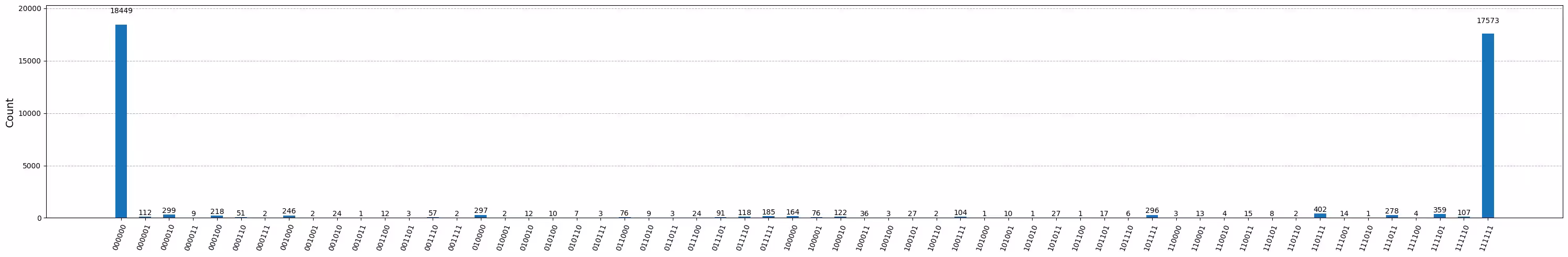
Ini adalah hasil Circuit GHZ 6 qubit. Seperti yang anda lihat, keadaan semua $|0\rangle$ dan semua $|1\rangle$ memang mendominasi, tetapi ralat adalah ketara. Mari cuba lihat seberapa besar Circuit GHZ yang boleh anda buat dengan peranti Eagle, sambil masih mendapat keputusan di mana keadaan yang betul sekurang-kurangnya lebih daripada 50% berkemungkinan.

1.2 Matlamat anda

Bina Circuit GHZ untuk 20 qubit atau lebih supaya, semasa pengukuran, kesetiaan keadaan GHZ anda > 0.5. Nota:

• Anda perlu menggunakan peranti Eagle (min_num_qubits=127) dan tetapkan bilangan shots sebagai 40,000.
• Anda perlu melaksanakan Circuit GHZ menggunakan fungsi execute_ghz_fidelity, dan mengira kesetiaan menggunakan fungsi check_ghz_fidelity_from_jobs.

Ini dimaksudkan sebagai latihan bebas, di mana anda memanfaatkan apa yang telah anda pelajari setakat ini dalam kursus ini.

def execute_ghz_fidelity(
    ghz_circuit: QuantumCircuit,  # Quantum circuit to create GHZ state (Circuit after Routing or without Routing), Classical register name is "c"
    physical_qubits: list[int],  # Physical qubits to represent GHZ state
    backend: BackendV2,
    sampler_options: dict | SamplerOptions | None = None,
):
    N_SHOTS = 40_000
    N = len(physical_qubits)
    base_circuit = ghz_circuit.remove_final_measurements(inplace=False)
    # M_k measurement circuits
    mk_circuits = []
    for k in range(1, N + 1):
        circuit = base_circuit.copy()
        # change measurement basis
        for q in physical_qubits:
            circuit.rz(-k * np.pi / N, q)
            circuit.h(q)
        mk_circuits.append(circuit)

    obs = SparsePauliOp.from_sparse_list(
        [("Z" * N, physical_qubits, 1)], num_qubits=backend.num_qubits
    )
    job_ids = []
    pm1 = generate_preset_pass_manager(1, backend=backend)
    org_transpiled = pm1.run(ghz_circuit)
    mk_transpiled = pm1.run(mk_circuits)
    with Batch(backend=backend):
        sampler = Sampler(options=sampler_options)
        sampler.options.twirling.enable_measure = True
        job = sampler.run([org_transpiled], shots=N_SHOTS)
        job_ids.append(job.job_id())
        # print(f"Sampler job id: {job.job_id()}, shots={N_SHOTS}")
        estimator = Estimator()  # TREX is applied as default
        estimator.options.dynamical_decoupling.enable = True
        estimator.options.execution.rep_delay = 0.0005
        estimator.options.twirling.enable_measure = True
        job2 = estimator.run([(circ, obs) for circ in mk_transpiled], precision=1 / 100)
        job_ids.append(job2.job_id())
        # print("Estimator job id:", job2.job_id())
        return [job.job_id(), job2.job_id()]

def check_ghz_fidelity_from_jobs(
    sampler_job,
    estimator_job,
    num_qubits,
    shots=40_000,
):
    N = num_qubits
    sampler_result = sampler_job.result()
    counts = sampler_result[0].data.c.get_counts()
    all_zero = counts.get("0" * N, 0) / shots
    all_one = counts.get("1" * N, 0) / shots
    top3 = sorted(counts, key=counts.get, reverse=True)[:3]
    print(
        f"N={N}: |00..0>: {counts.get('0'*N, 0)}, |11..1>: {counts.get('1'*N, 0)}, |3rd>: {counts.get(top3[2], 0)} ({top3[2]})"
    )
    print(f"P(|00..0>)={all_zero}, P(|11..1>)={all_one}")

    estimator_result = estimator_job.result()
    non_diagonal = (1 / N) * sum(
        (-1) ** k * estimator_result[k - 1].data.evs for k in range(1, N + 1)
    )
    print(f"REM: Coherence (non-diagonal): {non_diagonal:.6f}")
    fidelity = 0.5 * (all_zero + all_one + non_diagonal)
    sigma = 0.5 * np.sqrt(
        (1 - all_zero - all_one) * (all_zero + all_one) / shots
        + sum(estimator_result[k].data.stds ** 2 for k in range(N)) / (N * N)
    )
    print(f"GHZ fidelity = {fidelity:.6f} ± {sigma:.6f}")
    if fidelity - 2 * sigma > 0.5:
        print("GME (genuinely multipartite entangled) test: Passed")
    else:
        print("GME (genuinely multipartite entangled) test: Failed")
    return {
        "fidelity": fidelity,
        "sigma": sigma,
        "shots": shots,
        "job_ids": [sampler_job.job_id(), estimator_job.job_id()],
    }

Dalam buku nota ini, kita akan menerapkan tiga strategi untuk mencipta keadaan GHZ yang baik menggunakan 16 qubit dan 30 qubit. Pendekatan ini dibina berdasarkan strategi yang telah anda ketahui daripada pelajaran sebelumnya.

2. Strategi 1. Pemilihan Qubit Sedar Hingar

Kita mula dengan menentukan satu backend. Oleh kerana kita akan bekerja secara intensif dengan sifat-sifat sebuah backend tertentu, adalah lebih baik untuk menetapkan satu backend sahaja berbanding menggunakan pilihan least_busy.

backend = service.backend("ibm_strasbourg")  # eagle
twoq_gate = "ecr"
print(f"Device {backend.name} Loaded with {backend.num_qubits} qubits")
print(f"Two Qubit Gate: {twoq_gate}")

Device ibm_strasbourg Loaded with 127 qubits
Two Qubit Gate: ecr

Kita akan membina Circuit yang melibatkan banyak Gate dua-Qubit. Adalah masuk akal untuk menggunakan Qubit yang mempunyai ralat paling rendah semasa melaksanakan Gate dua-Qubit tersebut. Mencari "rantai Qubit" terbaik berdasarkan ralat Gate 2q yang dilaporkan merupakan masalah yang tidak mudah. Namun, kita boleh menakrifkan beberapa fungsi untuk membantu kita menentukan Qubit terbaik yang perlu digunakan.

coupling_map = backend.target.build_coupling_map(twoq_gate)
G = coupling_map.graph

def to_edges(path):  # create edges list from node paths
    edges = []
    prev_node = None
    for node in path:
        if prev_node is not None:
            if G.has_edge(prev_node, node):
                edges.append((prev_node, node))
            else:
                edges.append((node, prev_node))
        prev_node = node
    return edges

def path_fidelity(path, correct_by_duration: bool = True, readout_scale: float = None):
    """Compute an estimate of the total fidelity of 2-qubit gates on a path.
    If `correct_by_duration` is true, each gate fidelity is worsen by
    scale = max_duration / duration, that is, gate_fidelity^scale.
    If `readout_scale` > 0 is supplied, readout_fidelity^readout_scale
    for each qubit on the path is multiplied to the total fielity.
    The path is given in node indices form, for example, [0, 1, 2].
    An external function `to_edges` is used to obtain edge list, for example, [(0, 1), (1, 2)]."""
    path_edges = to_edges(path)
    max_duration = max(backend.target[twoq_gate][qs].duration for qs in path_edges)

    def gate_fidelity(qpair):
        duration = backend.target[twoq_gate][qpair].duration
        scale = max_duration / duration if correct_by_duration else 1.0
        # 1.25 = (d+1)/d with d = 4
        return max(0.25, 1 - (1.25 * backend.target[twoq_gate][qpair].error)) ** scale

    def readout_fidelity(qubit):
        return max(0.25, 1 - backend.target["measure"][(qubit,)].error)

    total_fidelity = np.prod(
        [gate_fidelity(qs) for qs in path_edges]
    )  # two qubits gate fidelity for each path
    if readout_scale:
        total_fidelity *= (
            np.prod([readout_fidelity(q) for q in path]) ** readout_scale
        )  # multiply readout fidelity
    return total_fidelity

def flatten(paths, cutoff=None):  # cutoff is for not making run time too large
    return [
        path
        for s, s_paths in paths.items()
        for t, st_paths in s_paths.items()
        for path in st_paths[:cutoff]
        if s < t
    ]

N = 16  # Number of qubits to use in the GHZ circuit
num_qubits_in_chain = N

Kita akan menggunakan fungsi-fungsi di atas untuk mencari semua laluan mudah N Qubit antara semua pasang nod dalam graf (Rujukan: all_pairs_all_simple_paths).

Kemudian, menggunakan fungsi path_fidelity yang dibuat di atas, kita akan mencari rantai Qubit terbaik yang mempunyai kesetiaan laluan paling tinggi.

from functools import partial

%%time
paths = rx.all_pairs_all_simple_paths(
    G.to_undirected(multigraph=False),
    min_depth=num_qubits_in_chain,
    cutoff=num_qubits_in_chain,
)
paths = flatten(paths, cutoff=25)  # If you have time, you could set a larger cutoff.
if not paths:
    raise Exception(
        f"No qubit chain with length={num_qubits_in_chain} exists in {backend.name}. Try smaller num_qubits_in_chain."
    )

print(f"Selecting the best from {len(paths)} candidate paths")

best_qubit_chain = max(
    paths, key=partial(path_fidelity, correct_by_duration=True, readout_scale=1.0)
)
assert len(best_qubit_chain) == num_qubits_in_chain
print(f"Predicted (best possible) process fidelity: {path_fidelity(best_qubit_chain)}")

Selecting the best from 6046 candidate paths
Predicted (best possible) process fidelity: 0.8929026784775056
CPU times: user 284 ms, sys: 10.9 ms, total: 295 ms
Wall time: 295 ms

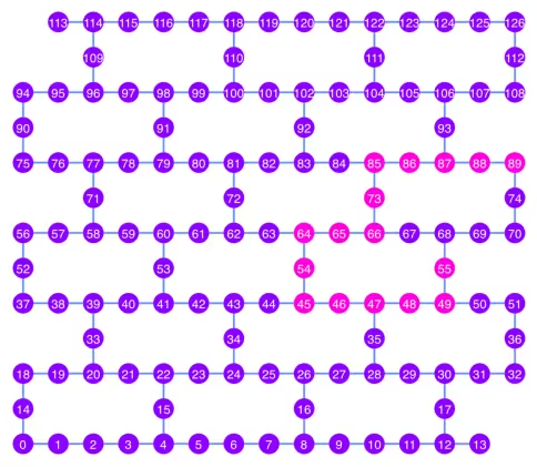
np.array(best_qubit_chain)

array([55, 49, 48, 47, 46, 45, 54, 64, 65, 66, 73, 85, 86, 87, 88, 89],
      dtype=uint64)

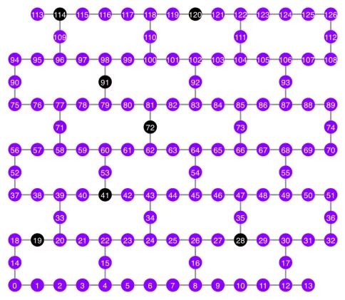
Mari kita plotkan rantai Qubit terbaik, yang ditunjukkan dalam warna merah jambu, dalam rajah peta gandingan.

qubit_color = []
for i in range(133):
    if i in best_qubit_chain:
        qubit_color.append("#ff00dd")  # pink
    else:
        qubit_color.append("#8c00ff")  # purple
plot_gate_map(
    backend, qubit_color=qubit_color, qubit_size=50, font_size=25, figsize=(6, 6)
)

2.1 Bina Circuit GHZ pada rantai Qubit terbaik

Kita pilih satu Qubit di tengah-tengah rantai untuk mengaplikasikan Gate H terlebih dahulu. Ini sepatutnya mengurangkan kedalaman Circuit hingga kira-kira separuh.

ghz1 = QuantumCircuit(max(best_qubit_chain) + 1, N)
ghz1.h(best_qubit_chain[N // 2])
for i in range(N // 2, 0, -1):
    ghz1.cx(best_qubit_chain[i], best_qubit_chain[i - 1])
for i in range(N // 2, N - 1, +1):
    ghz1.cx(best_qubit_chain[i], best_qubit_chain[i + 1])
ghz1.barrier()  # for visualization
ghz1.measure(best_qubit_chain, list(range(N)))
ghz1.draw(output="mpl", idle_wires=False, scale=0.5, fold=-1)

ghz1.depth()

10

pm = generate_preset_pass_manager(1, backend=backend)
ghz1_transpiled = pm.run(ghz1)
ghz1_transpiled.draw(output="mpl", idle_wires=False, fold=-1)

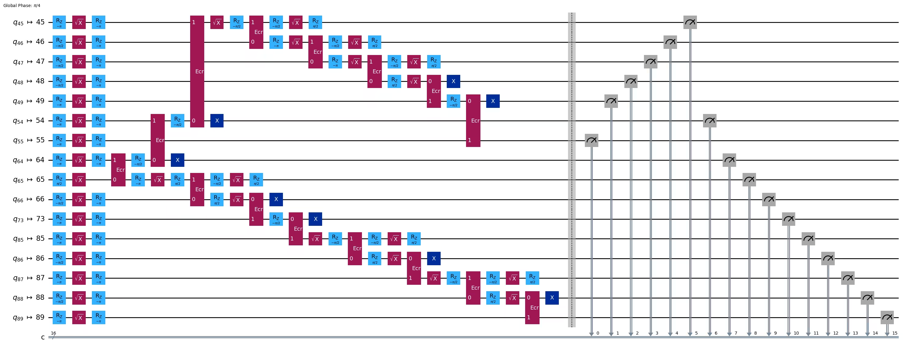
print("Depth:", ghz1_transpiled.depth())
print(
    "Two-qubit Depth:",
    ghz1_transpiled.depth(filter_function=lambda x: x.operation.num_qubits == 2),
)

Depth: 27
Two-qubit Depth: 8

opts = SamplerOptions()

res = execute_ghz_fidelity(
    ghz_circuit=ghz1,
    physical_qubits=best_qubit_chain,
    backend=backend,
    sampler_options=opts,
)

job_s = service.job(res[0])  # Use your job id showed above.
job_e = service.job(res[1])
print(job_s.status(), job_e.status())

DONE DONE

Berhati-hati untuk melaksanakan sel seterusnya selepas status kerja di atas menjadi 'DONE', bagi memaparkan keputusan menggunakan fungsi check_ghz_fidelity_from_jobs.

N = 16
# Check fidelity from job IDs
res = check_ghz_fidelity_from_jobs(
    sampler_job=job_s,
    estimator_job=job_e,
    num_qubits=N,
)

N=16: |00..0>: 153, |11..1>: 8681, |3rd>: 2262 (1111111111101111)
P(|00..0>)=0.003825, P(|11..1>)=0.217025
REM: Coherence (non-diagonal): 0.073809
GHZ fidelity = 0.147329 ± 0.002438
GME (genuinely multipartite entangled) test: Failed

result = job_s.result()
plot_histogram(result[0].data.c.get_counts(), figsize=(30, 5))

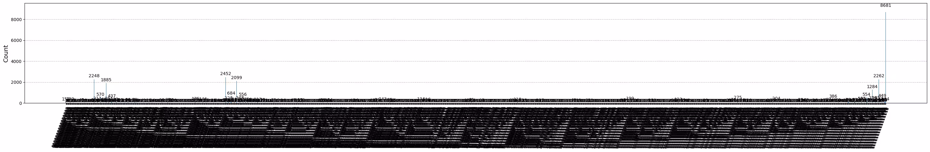
Keputusan ini tidak memenuhi kriteria. Mari kita beralih ke idea seterusnya.

3. Strategi 2. Pokok Qubit yang seimbang

Idea seterusnya ialah mencari pokok Qubit yang seimbang. Dengan menggunakan pokok berbanding rantaian, kedalaman Circuit sepatutnya menjadi lebih rendah. Sebelum itu, kita buang nod dengan ralat bacaan yang "teruk" dan tepi dengan ralat Gate yang "teruk" daripada graf penyambungan.

BAD_READOUT_ERROR_THRESHOLD = 0.1
BAD_ECRGATE_ERROR_THRESHOLD = 0.1
bad_readout_qubits = [
    q
    for q in range(backend.num_qubits)
    if backend.target["measure"][(q,)].error > BAD_READOUT_ERROR_THRESHOLD
]
bad_ecrgate_edges = [
    qpair
    for qpair in backend.target["ecr"]
    if backend.target["ecr"][qpair].error > BAD_ECRGATE_ERROR_THRESHOLD
]
print("Bad readout qubits:", bad_readout_qubits)
print("Bad ECR gates:", bad_ecrgate_edges)

Bad readout qubits: [19, 28, 41, 72, 91, 114, 120]
Bad ECR gates: []

g = backend.coupling_map.graph.copy().to_undirected()
g.remove_edges_from(
    bad_ecrgate_edges
)  # remove edge first (otherwise might fail with a NoEdgeBetweenNodes error)
g.remove_nodes_from(bad_readout_qubits)

Mari kita lukis graf peta penyambungan tanpa tepi yang teruk dan Qubit yang teruk.

qubit_color = []
for i in range(133):
    if i in bad_readout_qubits:
        qubit_color.append("#000000")  # black
    else:
        qubit_color.append("#8c00ff")  # purple
line_color = []
for e in backend.target.build_coupling_map().get_edges():
    if e in bad_ecrgate_edges:
        line_color.append("#ffffff")  # white
    else:
        line_color.append("#888888")  # gray
plot_gate_map(
    backend,
    qubit_color=qubit_color,
    line_color=line_color,
    qubit_size=50,
    font_size=25,
    figsize=(6, 6),
)

Kita cuba mencipta keadaan GHZ 16-Qubit seperti sebelumnya.

N = 16

Kita panggil fungsi betweenness_centrality untuk mencari Qubit bagi nod akar. Nod dengan nilai kepusatan kebersamaan (betweenness centrality) tertinggi berada di pusat graf. Rujukan: https://www.rustworkx.org/tutorial/betweenness_centrality.html

Atau anda boleh memilihnya secara manual.

# central = 65 #Select the center node manually
c_degree = dict(rx.betweenness_centrality(g))
central = max(c_degree, key=c_degree.get)
central

66

Bermula dari nod akar, jana pokok menggunakan carian mengikut lebar (BFS). Rujukan: https://qiskit.org/ecosystem/rustworkx/apiref/rustworkx.bfs_search.html#rustworkx-bfs-search

class TreeEdgesRecorder(rx.visit.BFSVisitor):
    def __init__(self, N):
        self.edges = []
        self.N = N

    def tree_edge(self, edge):
        self.edges.append(edge)
        if len(self.edges) >= self.N - 1:
            raise rx.visit.StopSearch()

vis = TreeEdgesRecorder(N)
rx.bfs_search(g, [central], vis)
best_qubits = sorted(list(set(q for e in vis.edges for q in (e[0], e[1]))))
# print('Tree edges:', vis.edges)

print("Qubits selected:", best_qubits)

Qubits selected: [54, 55, 63, 64, 65, 66, 67, 68, 69, 70, 73, 83, 84, 85, 86, 87]

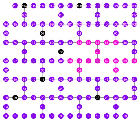
Mari kita plotkan Qubit yang dipilih, ditunjukkan dalam warna merah jambu, dalam gambar rajah peta penyambungan.

qubit_color = []
for i in range(133):
    if i in bad_readout_qubits:
        qubit_color.append("#000000")  # black
    elif i in best_qubits:
        qubit_color.append("#ff00dd")  # pink
    else:
        qubit_color.append("#8c00ff")  # purple
plot_gate_map(
    backend,
    qubit_color=qubit_color,
    line_color=line_color,
    qubit_size=50,
    font_size=25,
    figsize=(6, 6),
)

Mari kita tunjukkan struktur pokok bagi Qubit.

from rustworkx.visualization import graphviz_draw

tree = rx.PyDiGraph()
tree.extend_from_weighted_edge_list(vis.edges)
tree.remove_nodes_from([n for n in range(max(best_qubits) + 1) if n not in best_qubits])

graphviz_draw(tree, method="dot")

ghz2 = QuantumCircuit(max(best_qubits) + 1, N)

ghz2.h(tree.edge_list()[0][0])  # apply H-gate to the root node
# Apply CNOT from the root node to the each edge.
for u, v in tree.edge_list():
    ghz2.cx(u, v)
ghz2.barrier()  # for visualization
ghz2.measure(best_qubits, list(range(N)))
ghz2.draw(output="mpl", idle_wires=False, scale=0.5)

ghz2.depth()

8

pm = generate_preset_pass_manager(1, backend=backend)
ghz2_transpiled = pm.run(ghz2)
ghz2_transpiled.draw(output="mpl", idle_wires=False, fold=-1)

print("Depth:", ghz2_transpiled.depth())
print(
    "Two-qubit Depth:",
    ghz2_transpiled.depth(filter_function=lambda x: x.operation.num_qubits == 2),
)

Depth: 22
Two-qubit Depth: 6

Kedalaman Circuit kini telah menjadi jauh lebih rendah berbanding dengan struktur rantaian.

res = execute_ghz_fidelity(
    ghz_circuit=ghz2,
    physical_qubits=best_qubits,
    backend=backend,
    sampler_options=opts,
)

job_s = service.job(res[0])  # Use your job id showed above.
job_e = service.job(res[1])
print(job_s.status(), job_e.status())

DONE DONE

N = 16
# Check fidelity from job IDs
res = check_ghz_fidelity_from_jobs(
    sampler_job=job_s,
    estimator_job=job_e,
    num_qubits=N,
)

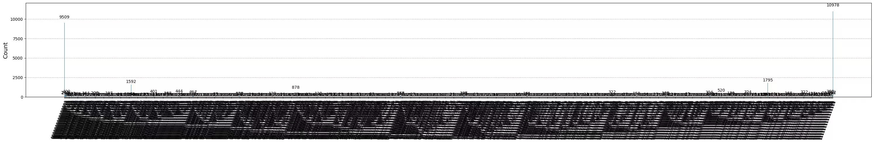
N=16: |00..0>: 9509, |11..1>: 10978, |3rd>: 1795 (1111110111111111)
P(|00..0>)=0.237725, P(|11..1>)=0.27445
REM: Coherence (non-diagonal): 0.606515
GHZ fidelity = 0.559345 ± 0.003188
GME (genuinely multipartite entangled) test: Passed

Kita berjaya lulus kriteria dengan struktur pokok yang seimbang!

result = job_s.result()
plot_histogram(result[0].data.c.get_counts(), figsize=(30, 5))

Sekarang, mari kita cuba mencipta keadaan GHZ yang lebih besar: keadaan GHZ 30-Qubit.

3.1 N = 30

Kita akan mengikuti kerangka corak Qiskit.

• Langkah 1: Petakan masalah kepada Circuit dan pengendali kuantum
• Langkah 2: Optimumkan untuk perkakasan sasaran
• Langkah 3: Laksanakan pada perkakasan sasaran
• Langkah 4: Proses keputusan pasca-pelaksanaan

Langkah 1: Petakan masalah kepada Circuit dan pengendali kuantum serta Langkah 2: Optimumkan untuk perkakasan sasaran

Di sini kita pilih nod akar secara manual.

central = 62  # Select the center node manually
# c_degree = dict(rx.betweenness_centrality(g))
# central = max(c_degree, key=c_degree.get)
# central

N = 30

vis = TreeEdgesRecorder(N)
rx.bfs_search(g, [central], vis)
best_qubits = sorted(list(set(q for e in vis.edges for q in (e[0], e[1]))))
print("Qubits selected:", best_qubits)

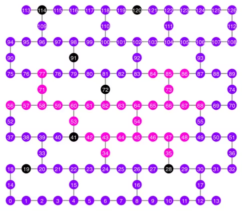
Qubits selected: [34, 35, 42, 43, 44, 45, 46, 47, 48, 53, 54, 56, 57, 58, 59, 60, 61, 62, 63, 64, 65, 66, 67, 68, 71, 73, 77, 84, 85, 86]

qubit_color = []
for i in range(133):
    if i in bad_readout_qubits:
        qubit_color.append("#000000")
    elif i in best_qubits:
        qubit_color.append("#ff00dd")
    else:
        qubit_color.append("#8c00ff")
line_color = []
for e in backend.target.build_coupling_map().get_edges():
    if e in bad_ecrgate_edges:
        line_color.append("#ffffff")
    else:
        line_color.append("#888888")
plot_gate_map(
    backend,
    qubit_color=qubit_color,
    line_color=line_color,
    qubit_size=50,
    font_size=25,
    figsize=(6, 6),
)

from rustworkx.visualization import graphviz_draw

tree = rx.PyDiGraph()
tree.extend_from_weighted_edge_list(vis.edges)
tree.remove_nodes_from([n for n in range(max(best_qubits) + 1) if n not in best_qubits])

graphviz_draw(tree, method="dot")

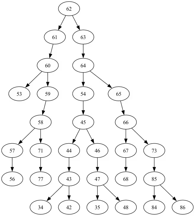
Kedalaman pokok ini ialah 5.

ghz3 = QuantumCircuit(max(best_qubits) + 1, N)

ghz3.h(tree.edge_list()[0][0])  # apply H-gate to the root node
# Apply CNOT from the root node to the each edge.
for u, v in tree.edge_list():
    ghz3.cx(u, v)
ghz3.barrier()  # for visualization
ghz3.measure(best_qubits, list(range(N)))
ghz3.draw(output="mpl", idle_wires=False, fold=-1)

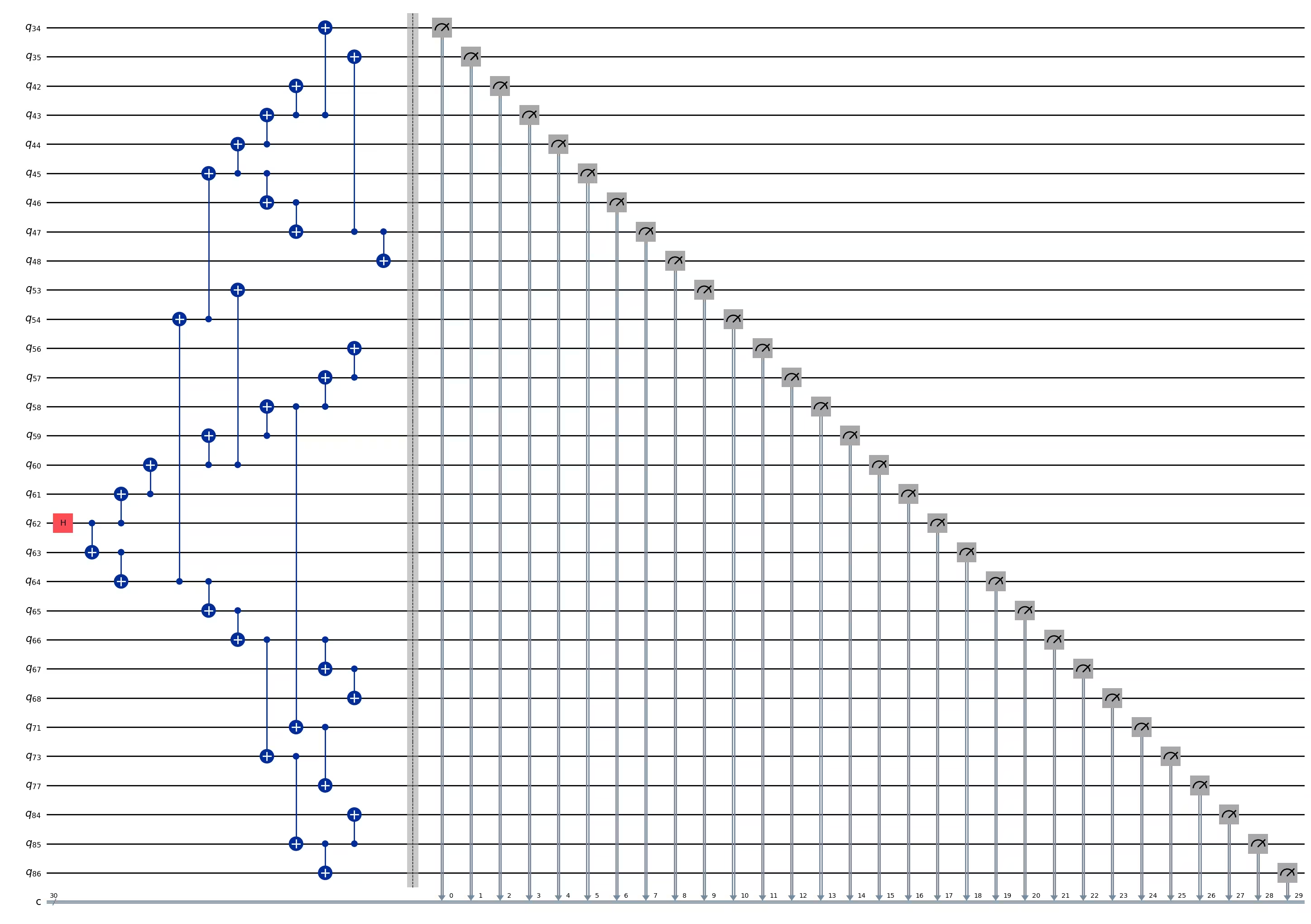
ghz3.depth()

11

pm = generate_preset_pass_manager(1, backend=backend)
ghz3_transpiled = pm.run(ghz3)
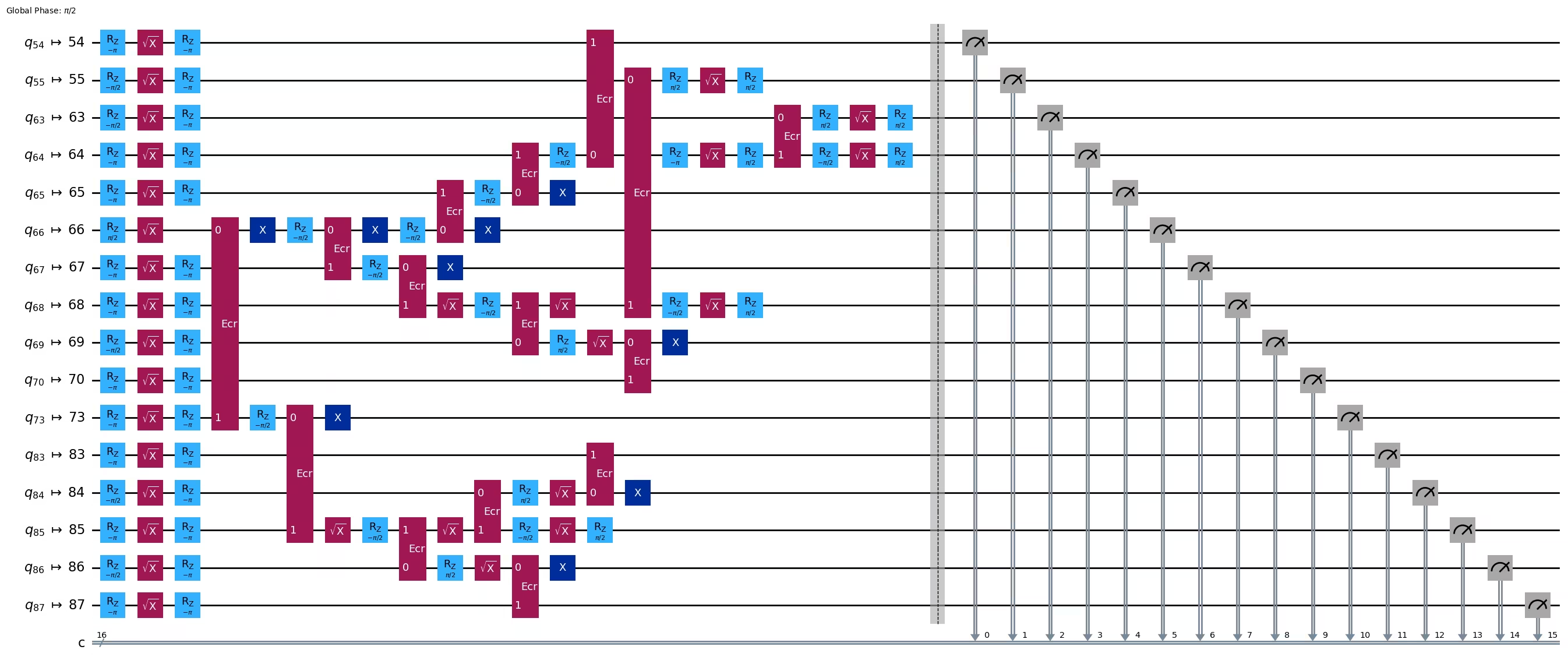
ghz3_transpiled.draw(output="mpl", idle_wires=False, fold=-1)

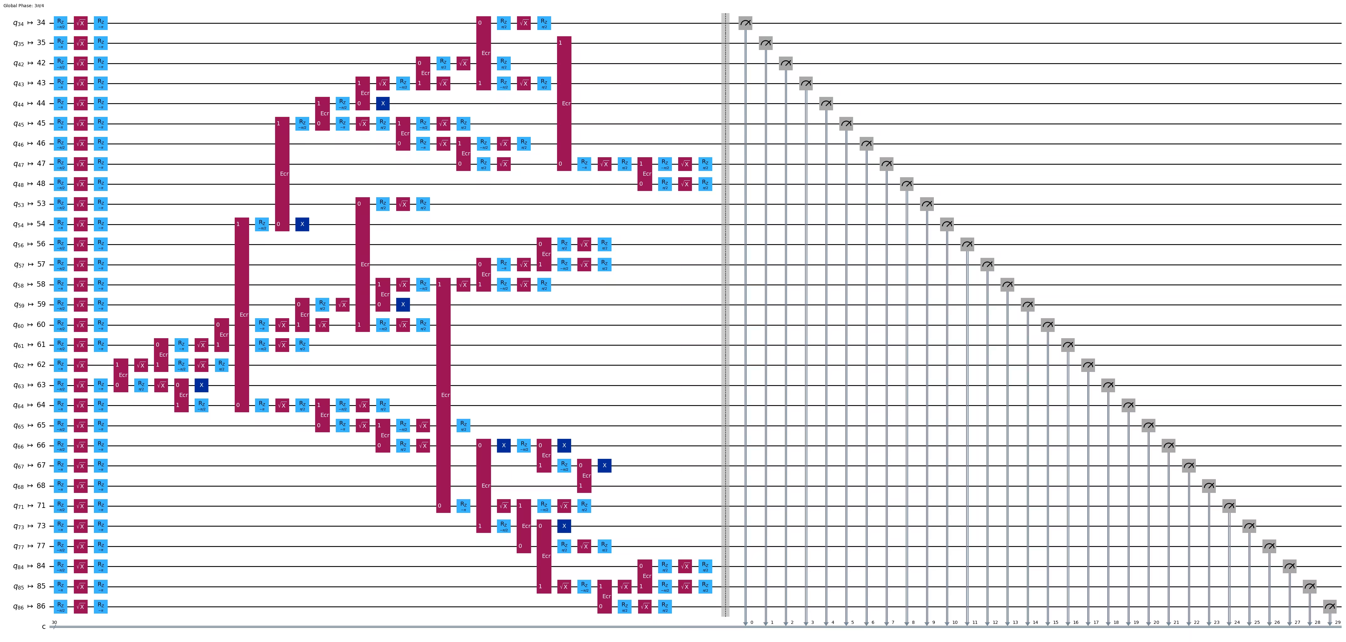
print("Depth:", ghz3_transpiled.depth())
print(
    "Two-qubit Depth:",
    ghz3_transpiled.depth(filter_function=lambda x: x.operation.num_qubits == 2),
)

Depth: 31
Two-qubit Depth: 9

3.2 Pilih nod akar yang berbeza secara manual

central = 54

vis = TreeEdgesRecorder(N)
rx.bfs_search(g, [central], vis)
best_qubits = sorted(list(set(q for e in vis.edges for q in (e[0], e[1]))))
print("Qubits selected:", best_qubits)

Qubits selected: [23, 24, 25, 34, 35, 42, 43, 44, 45, 46, 47, 48, 49, 50, 54, 55, 60, 61, 62, 63, 64, 65, 66, 67, 68, 69, 73, 84, 85, 86]

from rustworkx.visualization import graphviz_draw

tree = rx.PyDiGraph()
tree.extend_from_weighted_edge_list(vis.edges)
tree.remove_nodes_from([n for n in range(max(best_qubits) + 1) if n not in best_qubits])

graphviz_draw(tree, method="dot")

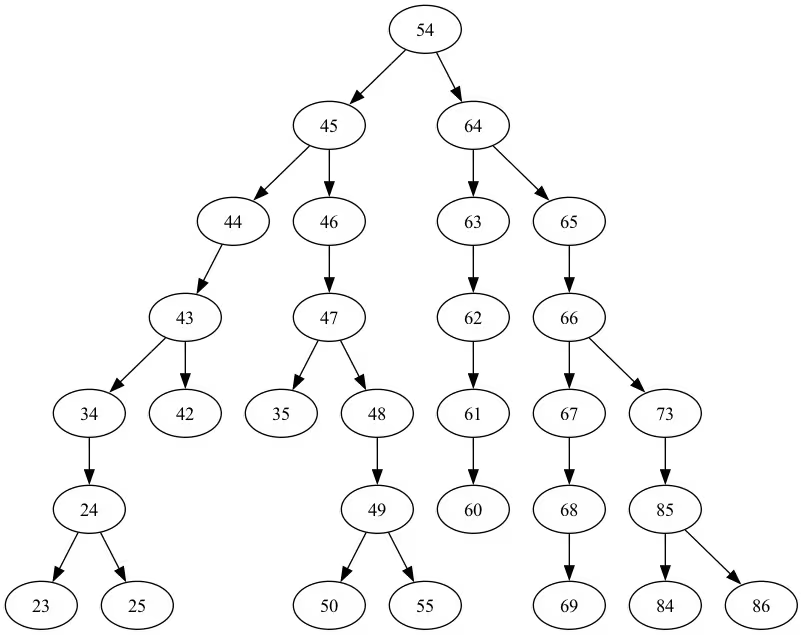
Kedalaman pokok ini ialah 6.

ghz3 = QuantumCircuit(max(best_qubits) + 1, N)

ghz3.h(tree.edge_list()[0][0])  # apply H-gate to the root node
# Apply CNOT from the root node to the each edge.
for u, v in tree.edge_list():
    ghz3.cx(u, v)
ghz3.barrier()  # for visualization
ghz3.measure(best_qubits, list(range(N)))
ghz3.draw(output="mpl", idle_wires=False, fold=-1)

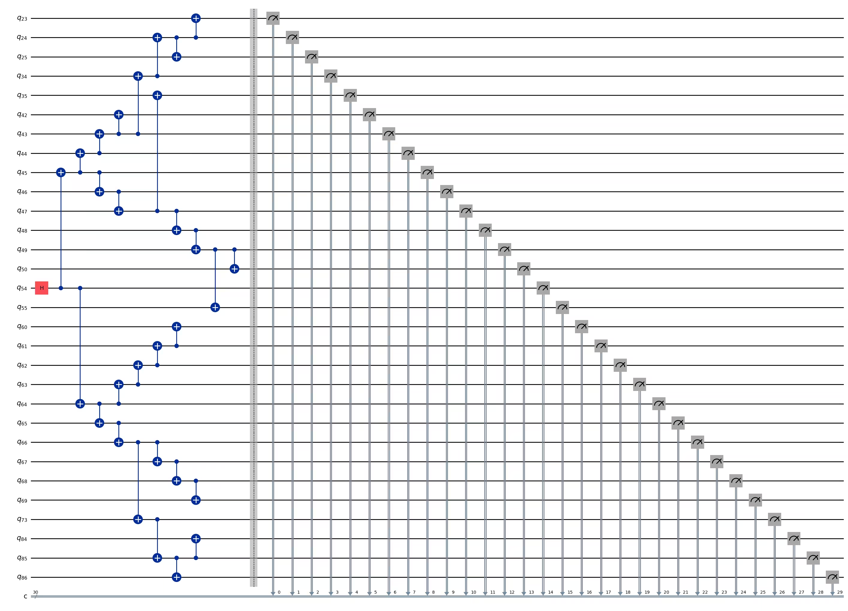
ghz3.depth()

11

pm = generate_preset_pass_manager(1, backend=backend)
ghz3_transpiled = pm.run(ghz3)
ghz3_transpiled.draw(output="mpl", idle_wires=False, fold=-1)

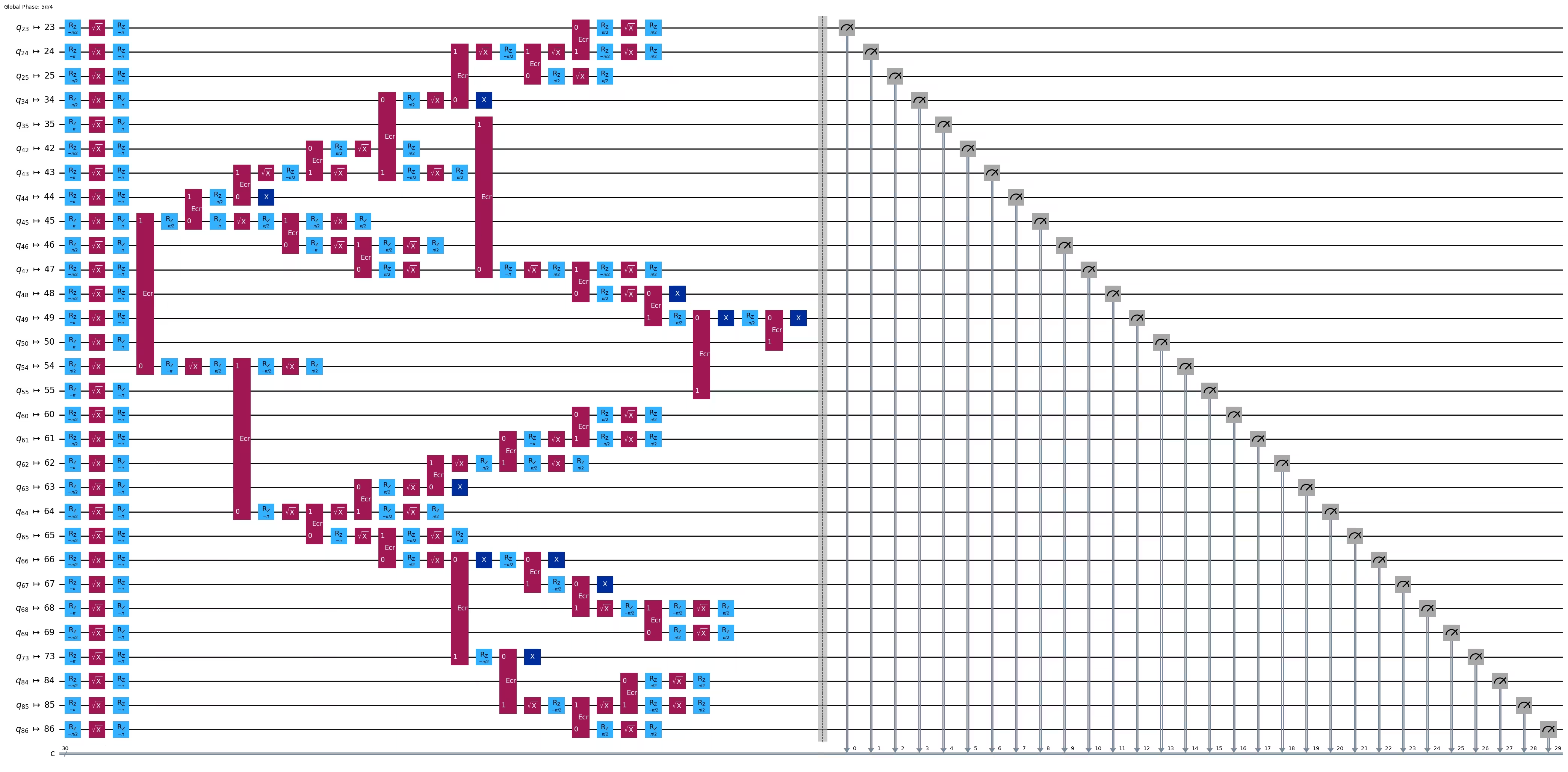
print("Depth:", ghz3_transpiled.depth())
print(
    "Two-qubit Depth:",
    ghz3_transpiled.depth(filter_function=lambda x: x.operation.num_qubits == 2),
)

Depth: 30
Two-qubit Depth: 9

Sungguh mengejutkan, walaupun kedalaman pokok meningkat dari 5 ke 6, kedalaman dua-Qubit berkurang dari 9 ke 8! Jadi mari kita gunakan Circuit yang terakhir ini.

Langkah 3: Laksanakan pada perkakasan sasaran

res = execute_ghz_fidelity(
    ghz_circuit=ghz3,
    physical_qubits=best_qubits,
    backend=backend,
    sampler_options=opts,
)

job_s = service.job(res[0])  # Use your job id showed above.
job_e = service.job(res[1])
print(job_s.status(), job_e.status())

DONE DONE

Langkah 4: Proses keputusan pasca-pelaksanaan

N = 30
# Check fidelity from job IDs
res = check_ghz_fidelity_from_jobs(
    sampler_job=job_s,
    estimator_job=job_e,
    num_qubits=N,
)

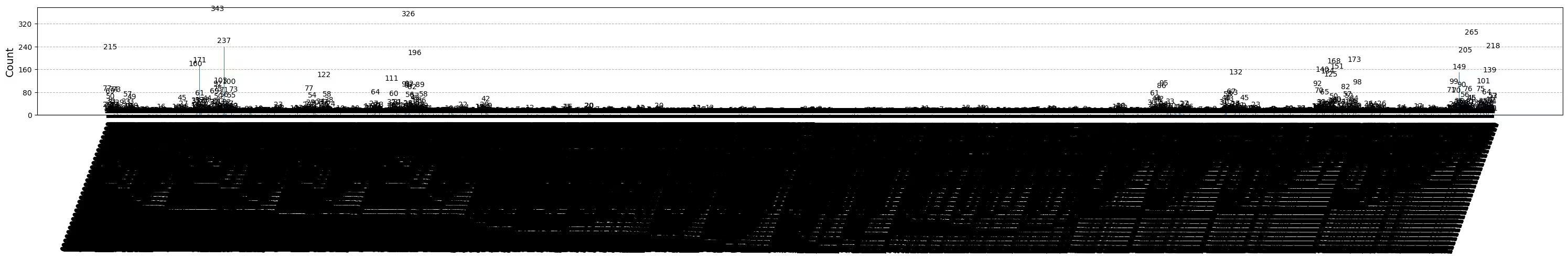
N=30: |00..0>: 4, |11..1>: 218, |3rd>: 265 (111111111111111011111111111111)
P(|00..0>)=0.0001, P(|11..1>)=0.00545
REM: Coherence (non-diagonal): 0.187073
GHZ fidelity = 0.096312 ± 0.003254
GME (genuinely multipartite entangled) test: Failed

Seperti yang anda lihat, keputusan ini tidak memenuhi kriteria.

# It will take some time
result = job_s.result()
plot_histogram(result[0].data.c.get_counts(), figsize=(30, 5))

4. Strategi 3. Jalankan dengan pilihan penindasan ralat

Anda boleh tetapkan pilihan penindasan ralat dalam Sampler V2. Rujuk panduan Konfigurasi pengurangan ralat dan rujukan API ExecutionOptionsV2 untuk maklumat lanjut.

opts = SamplerOptions()
opts.dynamical_decoupling.enable = True
opts.execution.rep_delay = 0.0005
opts.twirling.enable_gates = True

res = execute_ghz_fidelity(
    ghz_circuit=ghz3,
    physical_qubits=best_qubits,
    backend=backend,
    sampler_options=opts,
)

job_s = service.job(res[0])  # Use your job id showed above.
job_e = service.job(res[1])
print(job_s.status(), job_e.status())

DONE DONE

N = 30

# Check fidelity from job IDs
res = check_ghz_fidelity_from_jobs(
    sampler_job=job_s,
    estimator_job=job_e,
    num_qubits=N,
)

N=30: |00..0>: 1459, |11..1>: 1543, |3rd>: 359 (111111111111111111111111111110)
P(|00..0>)=0.036475, P(|11..1>)=0.038575
REM: Coherence (non-diagonal): 0.165532
GHZ fidelity = 0.120291 ± 0.003369
GME (genuinely multipartite entangled) test: Failed

# It will take some time
result = job_s.result()
plot_histogram(result[0].data.c.get_counts(), figsize=(30, 5))

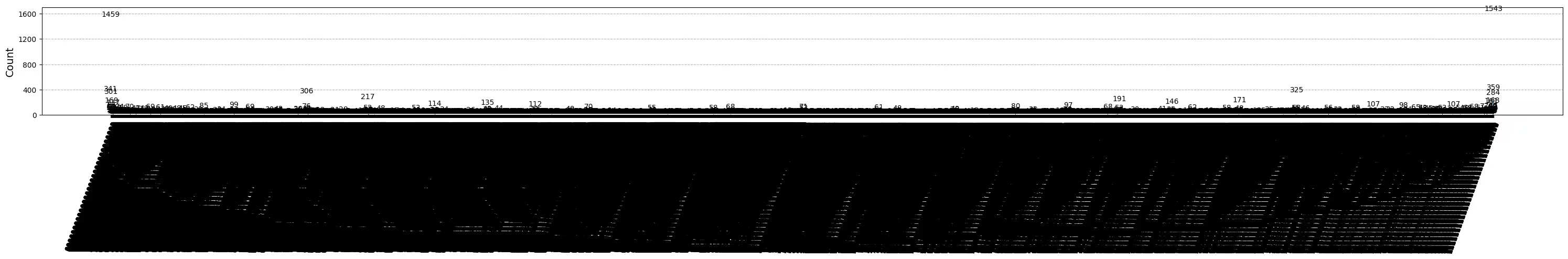
Keputusan telah bertambah baik tetapi masih belum memenuhi kriteria.

Kita telah melihat tiga idea setakat ini. Anda boleh menggabungkan dan mengembangkan idea-idea ini atau anda boleh mencetuskan idea sendiri untuk mencipta Circuit GHZ yang lebih baik. Sekarang mari kita semak semula matlamat tersebut.

5. Matlamat anda (ringkasan semula)

Bina Circuit GHZ untuk 20 Qubit atau lebih supaya keputusan pengukuran memenuhi kriteria: Kesetiaan keadaan GHZ anda > 0.5.

• Anda perlu menggunakan peranti Eagle (seperti ibm_brisbane) dan tetapkan bilangan tembakan sebagai 40,000.
• Anda perlu melaksanakan Circuit GHZ menggunakan fungsi execute_ghz_fidelity, dan mengira kesetiaan menggunakan fungsi check_ghz_fidelity_from_jobs.

Anda perlu mencari Circuit GHZ dengan bilangan Qubit terbesar yang memenuhi kriteria. Tulis kod anda di bawah, tunjukkan keputusan dengan fungsi check_ghz_fidelity_from_jobs.

Sekarang kita laksanakan aliran kerja GHZ yang sama seperti dalam bahan sebelumnya, tetapi pada peranti Heron. Ini memberi anda pengalaman dengan susun atur dan ciri-ciri pemproses Heron. Tiada strategi baru diperkenalkan.

Anggaran masa QPU untuk menjalankan eksperimen seterusnya ini ialah 4 minit 40 saat.

service = QiskitRuntimeService()
backend = service.backend("ibm_kingston")
# backend = service.backend("ibm_fez")

twoq_gate = "cz"
print(f"Device {backend.name} Loaded with {backend.num_qubits} qubits")
print(f"Two Qubit Gate: {twoq_gate}")

Device ibm_kingston Loaded with 156 qubits
Two Qubit Gate: cz

BAD_READOUT_ERROR_THRESHOLD = 0.1
BAD_CZGATE_ERROR_THRESHOLD = 0.1
bad_readout_qubits = [
    q
    for q in range(backend.num_qubits)
    if backend.target["measure"][(q,)].error > BAD_READOUT_ERROR_THRESHOLD
]
bad_czgate_edges = [
    qpair
    for qpair in backend.target["cz"]
    if backend.target["cz"][qpair].error > BAD_CZGATE_ERROR_THRESHOLD
]
print("Bad readout qubits:", bad_readout_qubits)
print("Bad CZ gates:", bad_czgate_edges)

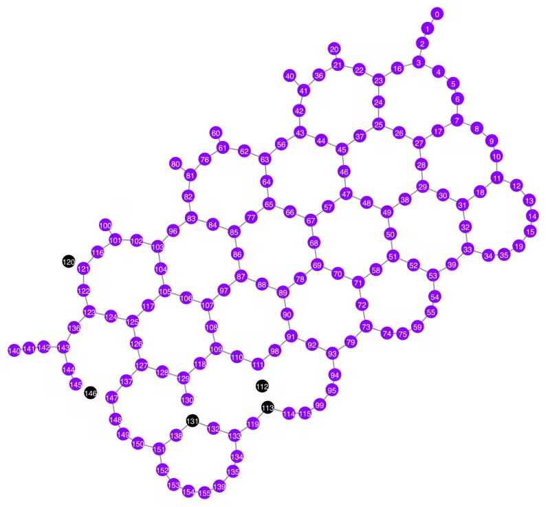
Bad readout qubits: [112, 113, 120, 131, 146]
Bad CZ gates: [(111, 112), (112, 111), (112, 113), (113, 112), (120, 121), (121, 120), (130, 131), (131, 130), (145, 146), (146, 145), (146, 147), (147, 146)]

g = backend.coupling_map.graph.copy().to_undirected()
g.remove_edges_from(
    bad_czgate_edges
)  # remove edge first (otherwise might fail with a NoEdgeBetweenNodes error)
g.remove_nodes_from(bad_readout_qubits)

qubit_color = []
for i in range(backend.num_qubits):
    if i in bad_readout_qubits:
        qubit_color.append("#000000")  # black
    else:
        qubit_color.append("#8c00ff")  # purple
line_color = []
for e in backend.target.build_coupling_map().get_edges():
    if e in bad_czgate_edges:
        line_color.append("#ffffff")  # white
    else:
        line_color.append("#888888")  # gray
plot_gate_map(
    backend,
    qubit_color=qubit_color,
    line_color=line_color,
    qubit_size=60,
    font_size=30,
    figsize=(10, 10),
)

N = 40
central = 100  # Select the center node manually
# c_degree = dict(rx.betweenness_centrality(g))
# central = max(c_degree, key=c_degree.get)
# central

class TreeEdgesRecorder(rx.visit.BFSVisitor):
    def __init__(self, N):
        self.edges = []
        self.N = N

    def tree_edge(self, edge):
        self.edges.append(edge)
        if len(self.edges) >= self.N - 1:
            raise rx.visit.StopSearch()

vis = TreeEdgesRecorder(N)
rx.bfs_search(g, [central], vis)
best_qubits = sorted(list(set(q for e in vis.edges for q in (e[0], e[1]))))
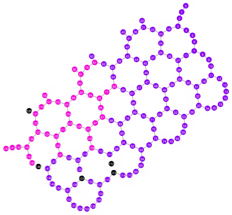
print("Qubits selected:", best_qubits)

Qubits selected: [61, 65, 76, 77, 80, 81, 82, 83, 84, 85, 86, 87, 96, 97, 100, 101, 102, 103, 104, 105, 106, 107, 108, 109, 116, 117, 121, 122, 123, 124, 125, 126, 127, 136, 140, 141, 142, 143, 144, 145]

qubit_color = []
for i in range(backend.num_qubits):
    if i in bad_readout_qubits:
        qubit_color.append("#000000")
    elif i in best_qubits:
        qubit_color.append("#ff00dd")
    else:
        qubit_color.append("#8c00ff")
line_color = []
for e in backend.target.build_coupling_map().get_edges():
    if e in bad_czgate_edges:
        line_color.append("#ffffff")
    else:
        line_color.append("#888888")
plot_gate_map(
    backend,
    qubit_color=qubit_color,
    line_color=line_color,
    qubit_size=60,
    font_size=30,
    figsize=(10, 10),
)

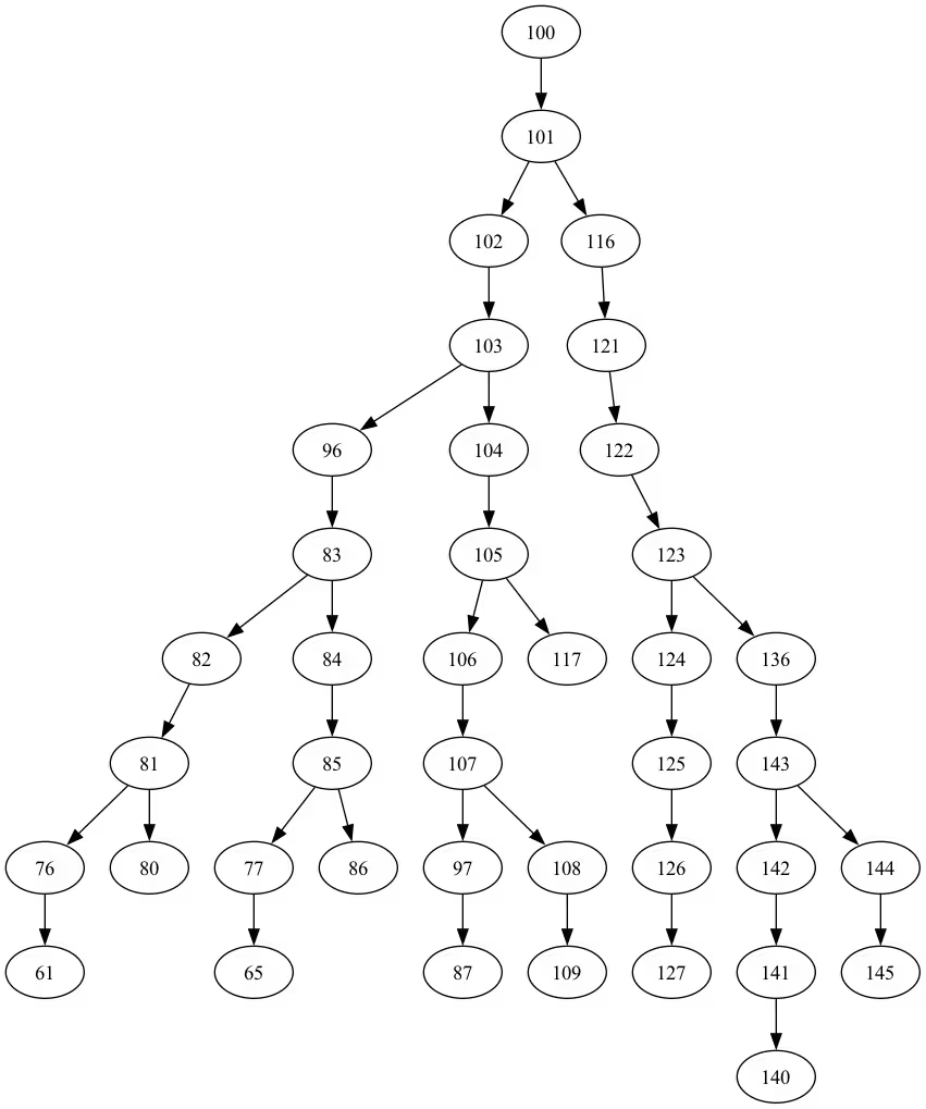
from rustworkx.visualization import graphviz_draw

tree = rx.PyDiGraph()
tree.extend_from_weighted_edge_list(vis.edges)
tree.remove_nodes_from([n for n in range(max(best_qubits) + 1) if n not in best_qubits])

graphviz_draw(tree, method="dot")

ghz_h = QuantumCircuit(max(best_qubits) + 1, N)

ghz_h.h(tree.edge_list()[0][0])  # apply H-gate to the root node
# Apply CNOT from the root node to the each edge.
for u, v in tree.edge_list():
    ghz_h.cx(u, v)
ghz_h.barrier()  # for visualization
ghz_h.measure(best_qubits, list(range(N)))
ghz_h.draw(output="mpl", idle_wires=False, fold=-1)

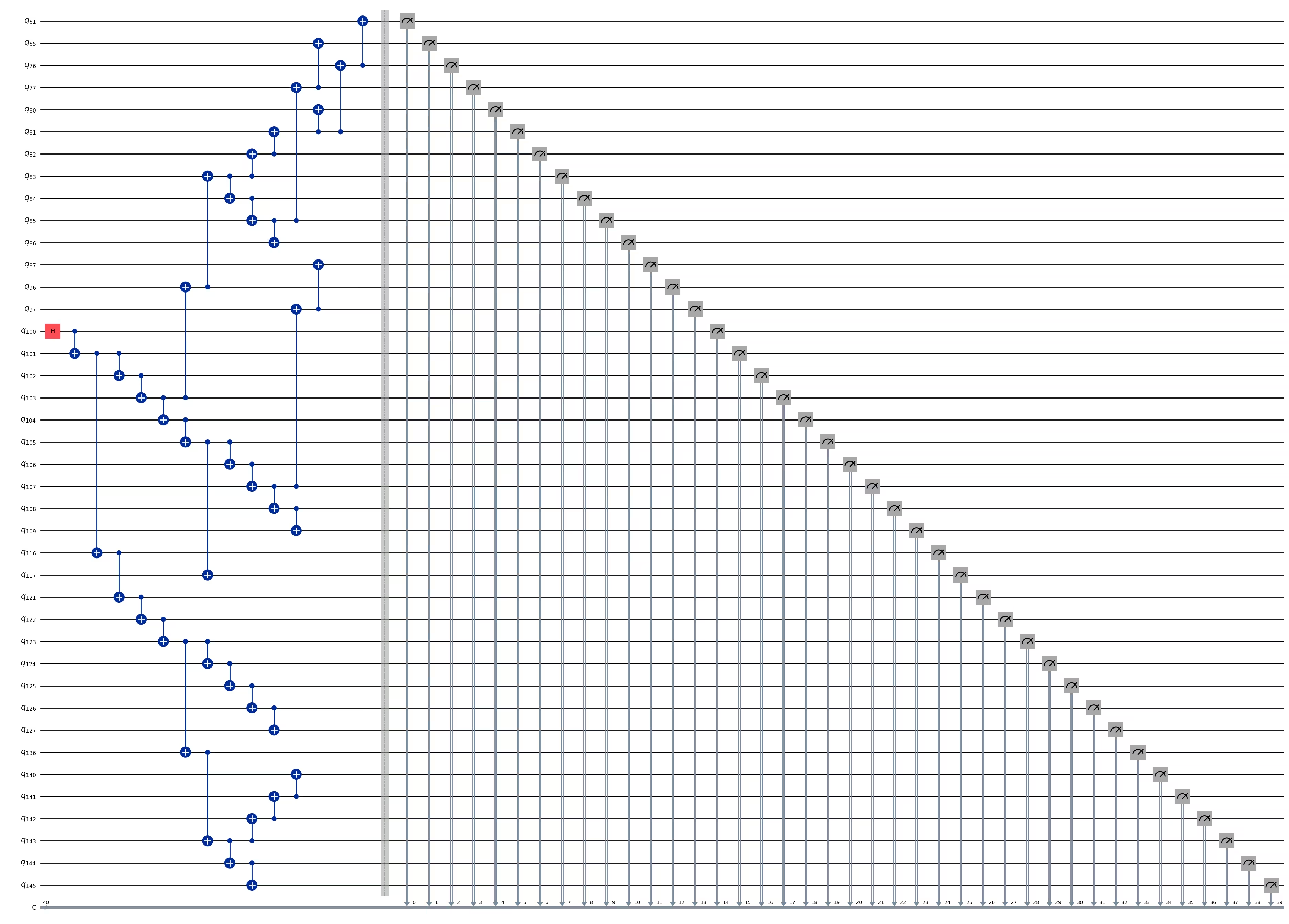
ghz_h.depth()

15

pm = generate_preset_pass_manager(1, backend=backend)
ghz_h_transpiled = pm.run(ghz_h)
ghz_h_transpiled.draw(output="mpl", idle_wires=False, fold=-1)

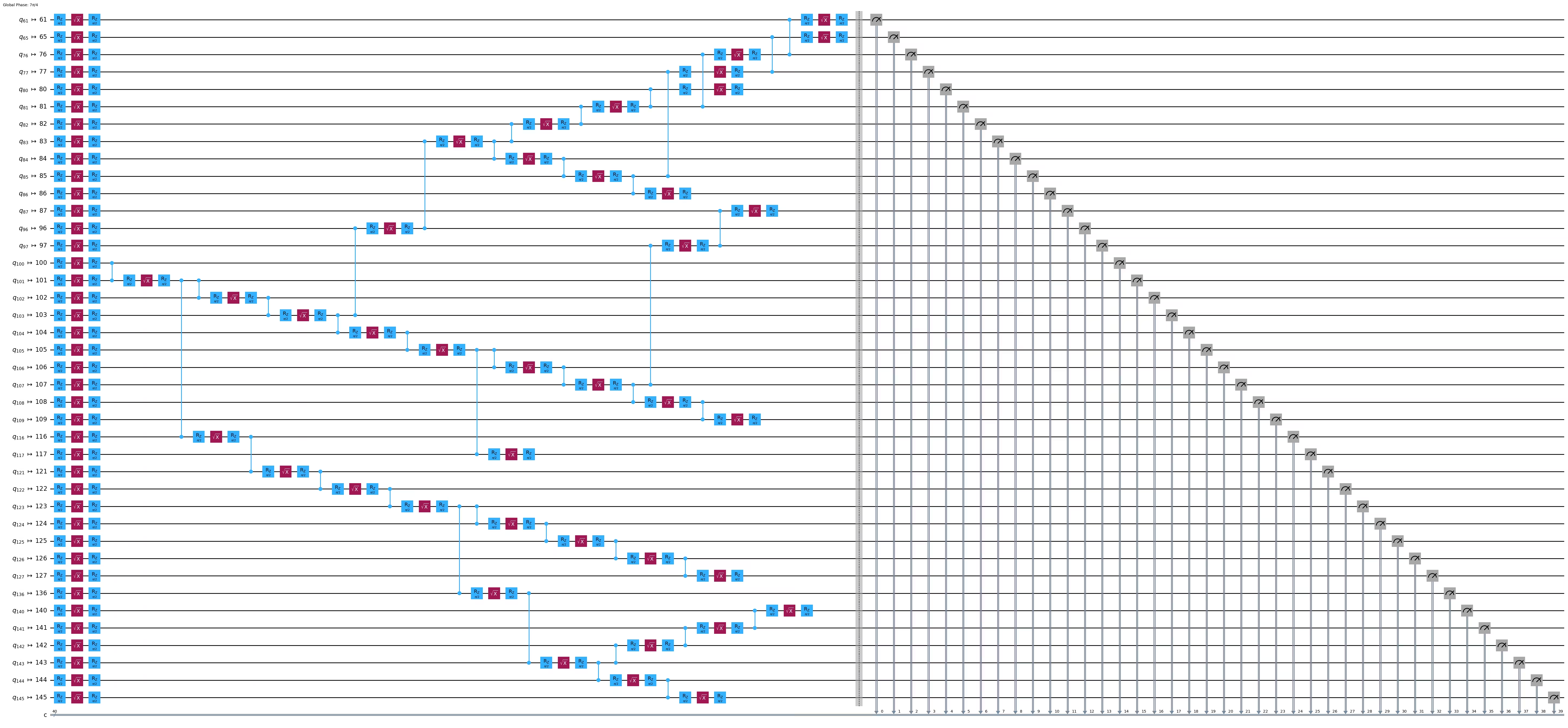
print("Depth:", ghz_h_transpiled.depth())
print(
    "Two-qubit Depth:",
    ghz_h_transpiled.depth(filter_function=lambda x: x.operation.num_qubits == 2),
)

Depth: 45
Two-qubit Depth: 13

opts = SamplerOptions()
opts.dynamical_decoupling.enable = True
opts.execution.rep_delay = 0.0005
opts.twirling.enable_gates = True

res = execute_ghz_fidelity(
    ghz_circuit=ghz_h,
    physical_qubits=best_qubits,
    backend=backend,
    sampler_options=opts,
)

job_s = service.job(res[0])  # Use your job id showed above.
job_e = service.job(res[1])
print(job_s.status(), job_e.status())

RUNNING RUNNING

# Check fidelity from job IDs
N = 40
res = check_ghz_fidelity_from_jobs(
    sampler_job=job_s,
    estimator_job=job_e,
    num_qubits=N,
)

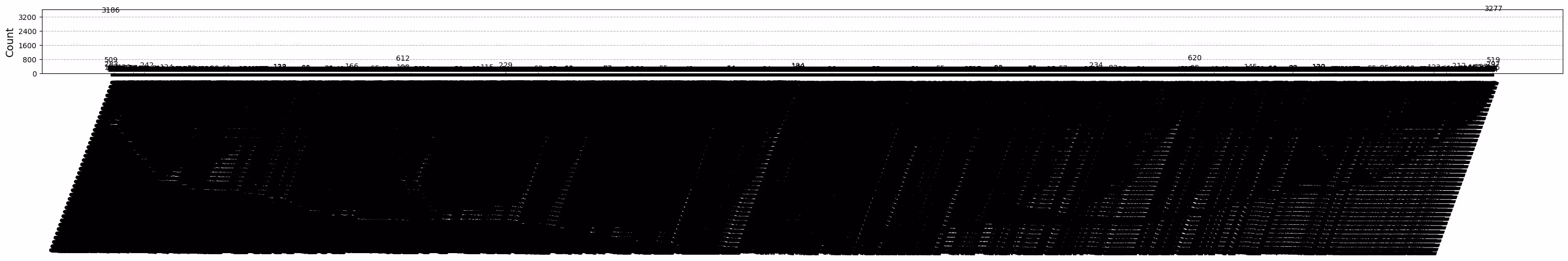
N=40: |00..0>: 3186, |11..1>: 3277, |3rd>: 620 (1111111011111111111111111111111111111111)
P(|00..0>)=0.07965, P(|11..1>)=0.081925
REM: Coherence (non-diagonal): 0.029987
GHZ fidelity = 0.095781 ± 0.002619
GME (genuinely multipartite entangled) test: Failed

# It will take some time
result = job_s.result()
plot_histogram(result[0].data.c.get_counts(), figsize=(30, 5))

Tahniah! Anda telah menyelesaikan pengenalan kepada pengkomputeran kuantum berskala utiliti! Anda kini bersedia untuk memberi sumbangan yang bermakna dalam pencarian kelebihan kuantum! Terima kasih kerana menjadikan IBM Quantum® sebahagian daripada perjalanan kuantum peribadi anda.

Kaji selidik pasca-kursus

Tahniah kerana berjaya menamatkan kursus ini! Sila luangkan masa untuk membantu kami memperbaiki kursus kami dengan mengisi kaji selidik ringkas berikut. Maklum balas anda akan digunakan untuk meningkatkan kandungan dan pengalaman pengguna kami. Terima kasih!

Note: This survey is provided by IBM Quantum and relates to the original English content. To give feedback on doQumentation's website, translations, or code execution, please open a GitHub issue.