Simulasi evolusi masa model Ising medan melintang

Anggaran penggunaan: 105 saat pada pemproses Nighthawk r2 (NOTA: Ini hanyalah anggaran. Masa larian anda mungkin berbeza.)

Hasil pembelajaran

Pelajari cara transpile dan menjalankan litar kuantum pada perkakasan menggunakan Julia
Pelajari cara pasca-proses hasil pengukuran untuk mengira nilai jangkaan
Pelajari cara membandingkan hasil perkakasan dengan simulasi klasik untuk mengukur kesan gabungan ralat penghampiran Trotter dan hingar perkakasan

Prasyarat

Biasakan diri dengan topik berikut sebelum memulakan tutorial ini:

Latar belakang

Julia ialah bahasa pengaturcaraan dinamik yang direka terutamanya untuk pengkomputeran berangka dan saintifik. Keupayaan pengkomputeran berangka berprestasi tingginya menjadikannya sesuai secara semula jadi untuk aliran kerja simulasi kuantum. Dalam tutorial ini, kami menunjukkan cara Julia digunakan untuk pra- dan pasca-pemprosesan klasik (contohnya, membina Hamiltonian, menjalankan penyelesai ODE (persamaan pembezaan biasa), dan mengira nilai jangkaan) dan untuk mengorkestra job perkakasan kuantum, menghapuskan keperluan untuk bertukar antara bahasa atau persekitaran.

Untuk berhubung dengan perkakasan IBM Quantum® daripada Julia, tutorial ini menggunakan dua pakej daripada ekosistem Qiskit: Qiskit.jl membungkus pustaka C Qiskit dan menyediakan fungsi pembinaan litar dan transpilasi dalam Julia; QiskitIBMRuntime.jl menyambung ke perkakasan IBM Quantum melalui klien IBM Quantum Compute Service, membolehkan penghantaran job dan pengambilan hasil terus daripada Julia.

Dalam tutorial ini, kita mempertimbangkan evolusi ter-Trotter bagi model Ising medan melintang pada rantai 1D dengan interaksi jiran terdekat:

H = \sum_{\langle i,j\rangle}J_{ij}Z_iZ_j + \sum_i h_i X_i

Untuk melaksanakan evolusi masa $e^{-iH\tau}$ , kita membahagikan sela masa $\tau$ kepada $r$ langkah dan mentakrifkan $\Delta\tau=\tau/r$ . Penguraian Trotter-Suzuki tertib kedua memberikan yang berikut:

e^{-iH\Delta\tau}\approx \prod_i e^{-ih_i X_i\Delta\tau/2 } \prod_{\langle i,j\rangle} e^{-iJ_{ij}Z_iZ_j\Delta\tau} \prod_i e^{-ih_iX_i\Delta\tau/2}

Untuk pembinaan litar, setiap langkah Trotter dilaksanakan sebagai urutan putaran $R_x$ satu-qubit dan gate $R_{ZZ}$ dua-qubit. Litar bermula dengan menyediakan keadaan Néel $|0101\cdots\rangle$ menggunakan gate X pada qubit berselang-seli. Setiap langkah Trotter berikutnya mengenakan: (1) $R_x(h_i\Delta\tau)$ pada setiap qubit, (2) $R_{ZZ}(2J_{ij}\Delta\tau)$ pada setiap pasangan berjiran di sepanjang rantai, dan (3) $R_x(h_i\Delta\tau)$ sekali lagi pada setiap qubit. Kedalaman litar keseluruhan bertambah secara linear dengan bilangan langkah Trotter $r$ .

Keperluan

Perhatikan bahawa tutorial ini memerlukan macOS atau Linux. Qiskit.jl buat masa ini tidak disokong pada Windows (dijejak dalam isu terbuka ini).

Untuk bermula, pasang Julia, dengan mengikut arahan pada halaman muat turun Julia. Tutorial ini dibangunkan dengan Julia 1.11; pasangnya dengan juliaup add 1.11.

Seterusnya, jalankan arahan berikut dalam terminal untuk memasang pakej Julia IJulia ke dalam persekitaran global, supaya anda boleh menjalankan Julia di dalam buku nota Jupyter.

julia -e 'using Pkg; Pkg.add("IJulia")'

Kita menggunakan pengurus pakej terbina dalam Julia untuk menyediakan persekitaran projek. Terdapat dua cara untuk menyediakan persekitaran.

Pilihan 1: persekitaran sementara. Anda boleh menjalankan sel kod berikut untuk menyediakan persekitaran sementara dan memasang pakej yang diperlukan;

Pilihan 2: hasilkan semula persekitaran teruji yang tepat. Tetapkan download_toml_files = true dalam sel di bawah. Sel ini akan memuat turun Project.toml dan Manifest.toml daripada repositori dokumentasi ke dalam folder env_tutorial/time-evolution/ bersebelahan buku nota ini, kemudian mengaktifkan persekitaran itu dan memasang versi pakej tepat yang direkodkannya. Fail projek menerangkan persekitaran pada peringkat tinggi, contohnya, bahagian [deps] menyenaraikan semua kebergantungan. Fail manifes memasukkan versi tepat bagi setiap pakej (termasuk kebergantungan tidak langsung), yang menjadikan persekitaran boleh diulang. Lihat dokumentasi Julia untuk butiran lanjut.

Kebergantungan berikut akan dipasang dalam persekitaran.

Untuk pembinaan dan pelaksanaan litar kuantum:

Qiskit.jl
QiskitIBMRuntime.jl

Untuk simulasi klasik:

OrdinaryDiffEq.jl
TensorNetworkQuantumSimulator.jl

Untuk pasca-pemprosesan hasil dan visualisasi:

StatsBase.jl
Plots.jl

Tutorial ini diuji dengan Qiskit.jl versi 0.6.0 dan QiskitIBMRuntime.jl versi 0.3.1.

using Pkg
using Downloads

download_toml_files = false

if !download_toml_files
    # Option 1: Install the latest versions of the required packages into a temporary environment
    Pkg.activate(mktempdir(); io=devnull)
    Pkg.add([
        PackageSpec(name="Qiskit"),
        PackageSpec(name="QiskitIBMRuntime"),
        PackageSpec(name="Python_jll"),
        PackageSpec(name="OrdinaryDiffEq"),
        PackageSpec(name="TensorNetworkQuantumSimulator"),
        PackageSpec(name="StatsBase"),
        PackageSpec(name="Plots"),
    ]; io=devnull)
else
    # Option 2: Install the exact tested versions pinned in the downloaded Project.toml and Manifest.toml
    base_url = "https://raw.githubusercontent.com/Qiskit/documentation/main/docs/tutorials/assets/time-evolution/julia"
    env_dir = joinpath(@__DIR__, "env_tutorial", "time-evolution")
    mkpath(env_dir)
    for file in ("Project.toml", "Manifest.toml")
        Downloads.download("$base_url/$file", joinpath(env_dir, file))
    end

    Pkg.activate(env_dir; io=devnull)
    Pkg.instantiate(; io=devnull) # installs the exact versions recorded in Manifest.toml
end

Sehingga ke tahap ini, kita telah menyediakan persekitaran projek Julia untuk menjalankan buku nota. Untuk menjalankan aliran kerja pada unit pemprosesan kuantum IBM, anda memerlukan akaun IBM Quantum dan token API untuk menginstansiasi perkhidmatan daripada qiskit-ibm-runtime. Ikut langkah "Install and authenticate" dalam topik Run your first circuit on hardware untuk menjana token API anda dan mencari CRN instans anda.

Persediaan

using Qiskit
using Qiskit.Operations
using QiskitIBMRuntime
using StatsBase
using OrdinaryDiffEq
using SparseArrays
using LinearAlgebra
using TensorNetworkQuantumSimulator
using Plots: plot, plot!, heatmap, @layout, mm

Kita juga mentakrifkan fungsi utiliti berikut, yang memulangkan nilai bit dalam bitstring v pada kedudukan i. Contohnya, dengan v = 6 (binari 110),

bit_at(6, 1) memulangkan 0,
bit_at(6, 2) memulangkan 1,
bit_at(6, 3) memulangkan 1.

Ini mengikut konvensyen little-endian yang digunakan dalam Qiskit: kedudukan i diindeks bermula dari bit paling tidak signifikan (bit "paling kanan").

"""
    bit_at(v::Integer, i::Integer) = (v >> (i-1)) & 1

Return the value of the bit at position `i` in `v`.
"""
bit_at(v::Integer, i::Integer) = (v >> (i-1)) & 1

bit_at

Contoh simulator berskala kecil

Kita pertimbangkan rantai 1D dengan $N$ qubit, yang diterangkan oleh model Ising medan melintang di atas. Untuk sistem yang dikaji, di bawah kita tetapkan saiz sistem N, saiz langkah Trotter δt, dan jumlah langkah Trotter r_max. Jumlah masa evolusi ialah δt * r_max. Perhatikan bahawa Julia menyokong pengecam Unicode seperti δt; dalam notebook atau Julia REPL, taip \delta diikuti Tab untuk memasukkan δ. Untuk rujukan penuh, lihat dokumentasi input Unicode Julia.

Penyelesaian tepat

Untuk menetapkan garis dasar bagi membandingkan hasil daripada perkakasan kuantum, mula-mula kita tunjukkan aliran kerja simulasi klasik untuk masalah berskala kecil. Kita bina Hamiltonian Ising sebagai matriks jarang, kemudian dapatkan evolusi masa yang tepat dengan mengamirkan persamaan Schrödinger secara berangka menggunakan ODEProblem daripada OrdinaryDiffEq.jl. Pendekatan ini berskala secara eksponen dengan bilangan qubit $N$ . Ia memerlukan penyimpanan vektor keadaan penuh berdimensi $2^N$ . Untuk $N=20$ , ruang Hilbert sudah mempunyai lebih sejuta dimensi, menjadikannya tidak praktikal untuk sistem yang lebih besar.

N = 20
δt = 0.05 # Trotter step size
r_max = 10 # total number of Trotter steps

h = fill(1.0, N)
J = fill(1.0, N-1)

# Build the Ising Hamiltonian as a sparse 2^n × 2^n matrix
function build_ising_hamiltonian(h::AbstractVector{<:Real}, J::AbstractVector{<:Real}, n::Int)
    dim = 2^n

    # diagonal ZZ terms
    diag_terms = zeros(Float64, dim)
    for i in 1:n-1
        for b in 0:dim-1
            bi = bit_at(b, i) # bit at position i
            bi_next = bit_at(b, i+1) # bit at position i + 1
            diag_terms[b+1] += J[i] * (1-2bi) * (1-2bi_next)
        end
    end
    H = spdiagm(0 => complex(diag_terms))

    # off-diagonal local X terms
    for i in 1:n
        mask = 1 << (i-1)
        cols = [xor(b, mask) + 1 for b in 0:dim-1]
        H += h[i] * sparse(1:dim, cols, ones(ComplexF64, dim), dim, dim)
    end
    return H
end

H_ising = build_ising_hamiltonian(h, J, N)

1048576×1048576 SparseMatrixCSC{ComplexF64, Int64} with 22020096 stored entries:
⎡⣿⣿⣾⢦⡀⠳⣄⠀⠀⠀⠳⣄⠀⠀⠀⠀⠀⠀⠀⠀⠳⣄⠀⠀⠀⠀⠀⠀⠀⠀⠀⠀⠀⠀⠀⠀⠀⠀⠀⠀⎤
⎢⠺⣟⢻⣶⣿⡂⠈⠳⣄⠀⠀⠈⠳⣄⠀⠀⠀⠀⠀⠀⠀⠈⠳⣄⠀⠀⠀⠀⠀⠀⠀⠀⠀⠀⠀⠀⠀⠀⠀⠀⎥
⎢⢤⡈⠻⠻⠿⣧⣤⣠⡈⠳⠄⠀⠀⠈⠳⣄⠀⠀⠀⠀⠀⠀⠀⠈⠳⣄⠀⠀⠀⠀⠀⠀⠀⠀⠀⠀⠀⠀⠀⠀⎥
⎢⠀⠙⢦⡀⠀⣻⣿⣿⣙⣦⡀⠀⠀⠀⠀⠈⠳⣄⠀⠀⠀⠀⠀⠀⠀⠈⠳⣄⠀⠀⠀⠀⠀⠀⠀⠀⠀⠀⠀⠀⎥
⎢⠀⠀⠀⠙⢦⡈⠳⣼⣿⣿⡆⠀⠀⠀⠀⠀⠀⠈⠳⣄⠀⠀⠀⠀⠀⠀⠀⠈⠳⣄⠀⠀⠀⠀⠀⠀⠀⠀⠀⠀⎥
⎢⠙⢦⡀⠀⠀⠁⠀⠈⠈⠉⣿⣿⣾⢦⡀⠳⣄⠀⠀⠈⠀⠀⠀⠀⠀⠀⠀⠀⠀⠈⠳⣄⠀⠀⠀⠀⠀⠀⠀⠀⎥
⎢⠀⠀⠙⢦⡀⠀⠀⠀⠀⠀⠺⣟⢻⣶⣿⡂⠈⠳⣄⠀⠀⠀⠀⠀⠀⠀⠀⠀⠀⠀⠀⠈⠳⣄⠀⠀⠀⠀⠀⠀⎥
⎢⠀⠀⠀⠀⠙⢦⡀⠀⠀⠀⢤⡈⠻⠻⠿⣧⣤⣠⡈⠳⠀⠀⠀⠀⠀⠀⠀⠀⠀⠀⠀⠀⠀⠈⠳⣄⠀⠀⠀⠀⎥
⎢⠀⠀⠀⠀⠀⠀⠙⢦⡀⠀⠀⠙⢦⡀⠀⣻⣿⣿⣙⣦⠀⠀⠀⠀⠀⠀⠀⠀⠀⠀⠀⠀⠀⠀⠀⠈⠳⣄⠀⠀⎥
⎢⠀⠀⠀⠀⠀⠀⠀⠀⠙⢦⡀⠀⠀⠙⢦⡈⠳⣼⣿⣿⠀⠀⠀⠀⠀⠀⠀⠀⠀⠀⠀⠀⠀⠀⠀⠀⠀⠈⠳⣄⎥
⎢⠙⢦⡀⠀⠀⠀⠀⠀⠀⠀⠀⠀⠀⠀⠀⠀⠀⠀⠀⠀⣿⣿⡟⢦⡈⠳⣄⠀⠀⠈⠳⣄⠀⠀⠀⠀⠀⠀⠀⠀⎥
⎢⠀⠀⠙⢦⡀⠀⠀⠀⠀⠀⠀⠀⠀⠀⠀⠀⠀⠀⠀⠀⠻⣍⣿⣿⣯⠀⠈⠳⣄⠀⠀⠈⠳⣄⠀⠀⠀⠀⠀⠀⎥
⎢⠀⠀⠀⠀⠙⢦⡀⠀⠀⠀⠀⠀⠀⠀⠀⠀⠀⠀⠀⠀⢦⡈⠋⠛⢻⣶⣦⣦⡈⠓⠀⠀⠀⠈⠳⣄⠀⠀⠀⠀⎥
⎢⠀⠀⠀⠀⠀⠀⠙⢦⡀⠀⠀⠀⠀⠀⠀⠀⠀⠀⠀⠀⠀⠙⢦⡀⠨⣿⠿⣧⣽⡦⠀⠀⠀⠀⠀⠈⠳⣄⠀⠀⎥
⎢⠀⠀⠀⠀⠀⠀⠀⠀⠙⢦⡀⠀⠀⠀⠀⠀⠀⠀⠀⠀⡀⠀⠀⠙⢦⠈⠳⡿⣿⣿⣀⡀⡀⠀⢀⠀⠀⠈⠳⣄⎥
⎢⠀⠀⠀⠀⠀⠀⠀⠀⠀⠀⠙⢦⡀⠀⠀⠀⠀⠀⠀⠀⠙⢦⡀⠀⠀⠀⠀⠀⠀⠸⣿⣿⡟⢦⡈⠳⣄⠀⠀⠀⎥
⎢⠀⠀⠀⠀⠀⠀⠀⠀⠀⠀⠀⠀⠙⢦⡀⠀⠀⠀⠀⠀⠀⠀⠙⢦⡀⠀⠀⠀⠀⠈⠻⣍⣿⣿⣯⠀⠈⠳⣄⠀⎥
⎢⠀⠀⠀⠀⠀⠀⠀⠀⠀⠀⠀⠀⠀⠀⠙⢦⡀⠀⠀⠀⠀⠀⠀⠀⠙⢦⡀⠀⠀⠐⢦⡈⠋⠛⢻⣶⣦⣦⡈⠓⎥
⎢⠀⠀⠀⠀⠀⠀⠀⠀⠀⠀⠀⠀⠀⠀⠀⠀⠙⢦⡀⠀⠀⠀⠀⠀⠀⠀⠙⢦⡀⠀⠀⠙⢦⡀⠨⣿⠿⣧⣽⡦⎥
⎣⠀⠀⠀⠀⠀⠀⠀⠀⠀⠀⠀⠀⠀⠀⠀⠀⠀⠀⠙⢦⠀⠀⠀⠀⠀⠀⠀⠀⠙⢦⠀⠀⠀⠙⢦⠈⠳⡿⣿⣿⎦

Kita takrifkan bahagian kanan persamaan Schrödinger dalam bentuk in-place schrodinger!(dψ, ψ, H, t), yang mengira $d\psi/dt = -iH\psi$ menggunakan pendaraban matriks-vektor jarang. Kemudian kita sediakan ODEProblem dengan keadaan Néel sebagai keadaan awal dan selesaikannya pada julat masa $[0, r \cdot \delta t]$ , sambil menyimpan keadaan pada setiap langkah masa $\delta t$ . Penyelesai yang digunakan ialah Tsit5(), kaedah Runge-Kutta eksplisit tertib keempat/kelima yang standard dan sesuai untuk masalah tidak kaku.

# initial state |0101...01⟩
ψ0 = zeros(ComplexF64, 2^N)
neel_index = sum(1 << (i-1) for i in 1:2:N)
ψ0[neel_index + 1] = 1.0

function schrodinger!(dψ::AbstractVector, ψ::AbstractVector, H::AbstractMatrix, t::Real)
    mul!(dψ, H, ψ)
    dψ .*= -im
end

tspan = (0.0, r_max * δt)
prob = ODEProblem(schrodinger!, ψ0, tspan, H_ising)
sol = solve(prob, Tsit5(), saveat=δt)

retcode: Success
Interpolation: 1st order linear
t: 11-element Vector{Float64}:
 0.0
 0.05
 0.1
 0.15
 0.2
 0.25
 0.3
 0.35
 0.4
 0.45
 0.5
u: 11-element Vector{Vector{ComplexF64}}:
 [0.0 + 0.0im, 0.0 + 0.0im, 0.0 + 0.0im, 0.0 + 0.0im, 0.0 + 0.0im, 0.0 + 0.0im, 0.0 + 0.0im, 0.0 + 0.0im, 0.0 + 0.0im, 0.0 + 0.0im  …  0.0 + 0.0im, 0.0 + 0.0im, 0.0 + 0.0im, 0.0 + 0.0im, 0.0 + 0.0im, 0.0 + 0.0im, 0.0 + 0.0im, 0.0 + 0.0im, 0.0 + 0.0im, 0.0 + 0.0im]
 [-7.612535273941705e-14 + 2.5737401150886516e-29im, 7.616818423232204e-14 - 1.6944517510822304e-12im, -8.565903349044157e-17 + 3.2368190823993794e-15im, -7.61682079584434e-14 - 1.078515326911689e-15im, 1.523363843119942e-13 - 1.6912125988569567e-12im, 3.5867824743714624e-11 + 5.083352813839524e-12im, -7.608249752495255e-14 - 4.317561743447096e-15im, 7.616820798431766e-14 - 1.6944516451719627e-12im, -8.570258514925147e-17 + 3.2384113624188233e-15im, -7.606534127496737e-14 - 5.398093819616815e-15im  …  -7.591102113501652e-14 - 7.55501666902211e-15im, 1.5233640806402347e-13 - 1.691212597789024e-12im, -4.283149391646935e-17 + 3.2390475588024777e-15im, -7.61253567131055e-14 - 4.319154099332238e-15im, 1.28498500555455e-16 + 4.773388002812907e-18im, -8.570258413862945e-17 + 3.2384113624488572e-15im, -7.612534879063769e-14 - 3.2390464923709225e-15im, 1.5233638826330585e-13 - 1.6912127047672224e-12im, -4.283149290692347e-17 + 3.237455101084436e-15im, -7.612535273941595e-14 - 1.8338992189508272e-31im]
 [-8.680854672628291e-11 - 3.427254579020333e-25im, 8.709110140864061e-11 - 8.699033104505336e-10im, -5.649235901782656e-13 + 8.601572275260816e-12im, -8.709221846767839e-11 - 2.859732693854631e-12im, 1.7418295344900034e-10 - 8.612608133903897e-10im, 8.41248317362033e-9 + 2.6096671235273274e-9im, -8.652487588621059e-11 - 1.1500395899126693e-11im, 8.709222358844944e-11 - 8.699014655672987e-10im, -5.669821718119223e-13 + 8.629638578162805e-12im, -8.641073444337035e-11 - 1.4395664161950265e-11im  …  -8.538755211456945e-11 - 2.0113079067784756e-11im, 1.7418407565004836e-10 - 8.612606969068827e-10im, -2.825548799186401e-13 + 8.640787361594646e-12im, -8.680873675466659e-11 - 1.152847038256832e-11im, 8.478635815548866e-13 + 8.382372443494577e-14im, -5.669819735592012e-13 + 8.629638588149376e-12im, -8.680836165042751e-11 - 8.640671375786309e-12im, 1.7418313902498964e-10 - 8.61262658275938e-10im, -2.82554682353394e-13 + 8.612701741862262e-12im, -8.680854672628374e-11 - 2.811149115586865e-25im]
 [-4.2861942928308275e-9 - 4.7678984538985196e-24im, 4.318192995176613e-9 - 2.8269371315624182e-8im, -6.395173522788358e-11 + 6.447233357075582e-10im, -4.318468070877377e-9 - 2.1364257686596578e-10im, 8.636571975410676e-9 - 2.7617721500979347e-8im, 1.7289660717976908e-7 + 8.480086489483005e-8im, -4.253920910159066e-9 - 8.649865429907717e-10im, 4.318470318624579e-9 - 2.826906169988642e-8im, -6.446071076018044e-11 + 6.495016281145607e-10im, -4.240844230135151e-9 - 1.0846764703342651e-9im  …  -4.124170626784771e-9 - 1.5115818225612714e-9im, 8.636849310525618e-9 - 2.7617681592276622e-8im, -3.199878870600196e-11 + 6.513863923787342e-10im, -4.2862418335791054e-9 - 8.697676141630365e-10im, 9.60478168658149e-11 + 1.4206678132640617e-11im, -6.446062402203318e-11 + 6.495016332435747e-10im, -4.286148929585427e-9 - 6.513467397401749e-10im, 8.636617557977306e-9 - 2.7618031117900408e-8im, -3.1998702345812497e-11 + 6.466014984949206e-10im, -4.286194292830829e-9 + 4.870909626742163e-24im]
 [-6.079348924748445e-8 + 6.709717322272516e-24im, 6.162943323939352e-8 - 2.9592110353110093e-7im, -1.6696556398383817e-9 + 1.2400459826013194e-8im, -6.164292787255694e-8 - 4.088131560944853e-9im, 1.2326810978249792e-7 - 2.832733452226872e-7im, 1.253532043962043e-6 + 8.875042569125039e-7im, -5.994408800994472e-8 - 1.6725258647088304e-8im, 6.164314112979357e-8 - 2.9591021577421156e-7im, -1.6948387141108349e-9 + 1.2572865374243683e-8im, -5.959595610442699e-8 - 2.1031419496566967e-8im  …  -5.651357562833814e-8 - 2.9192023780832225e-8im, 1.2328181992163385e-7 - 2.832706038202527e-7im, -8.359520177503641e-10 + 1.2640019589288568e-8im, -6.079590106381668e-8 - 1.689785040734888e-8im, 2.5106376181130386e-9 + 5.084778396177926e-10im, -1.6948306165735295e-9 + 1.2572866042727832e-8im, -6.079128573701664e-8 - 1.2637312624047932e-8im, 1.2327033399936622e-7 - 2.8328423313378375e-7im, -8.359439919088748e-10 + 1.2467163914771088e-8im, -6.079348924748447e-8 + 1.0331673240130025e-23im]
 [-4.193552407608965e-7 - 1.840220498495959e-23im, 4.2862657866184504e-7 - 1.605297190776032e-6im, -1.8502762435969943e-8 + 1.0856276308591437e-7im, -4.288690355597115e-7 - 3.554458373697522e-8im, 8.574220964863143e-7 - 1.4932465582703908e-6im, 4.849187224415274e-6 + 4.812233679729101e-6im, -4.098425461298137e-7 - 1.4745065418194435e-7im, 4.288753395920834e-7 - 1.6051467128773302e-6im, -1.896035285782807e-8 + 1.1102835700521827e-7im, -4.0588320553359593e-7 - 1.8611022850670223e-7im  …  -3.711838427223188e-7 - 2.569391306045151e-7im, 8.57670971098675e-7 - 1.4931825847645462e-6im, -9.271568570757063e-9 + 1.1197289579952942e-7im, -4.194005371452928e-7 - 1.4992045110994755e-7im, 2.787088237718031e-8 + 7.194933454521717e-9im, -1.8960118645415406e-8 + 1.1102838165568638e-7im, -4.193161709409199e-7 - 1.1191024844294344e-7im, 8.574617742181924e-7 - 1.4933970418540967e-6im, -9.271337900947239e-9 + 1.0949690324053836e-7im, -4.193552407608964e-7 + 1.6524848989693985e-22im]
 [-1.7823579016922897e-6 - 1.087640585040274e-21im, 1.840838369770109e-6 - 5.569854913729441e-6im, -1.1658899308162594e-7 + 5.632670364049069e-7im, -1.843111911436975e-6 - 1.8277839588324167e-7im, 3.6832950716080163e-6 - 4.979757871286645e-6im, 1.1823232043972897e-5 + 1.668138856075027e-5im, -1.7216192586061922e-6 - 7.718155525067347e-7im, 1.8432004842500001e-6 - 5.56872697042903e-6im, -1.209408931510706e-7 + 5.825677201706816e-7im, -1.6958321412209815e-6 - 9.789484717969276e-7im  …  -1.4727630743780977e-6 - 1.3421173522554028e-6im, 3.6856596566327488e-6 - 4.9790105233659736e-6im, -5.848359517965976e-8 + 5.898080282235565e-7im, -1.7828068643880377e-6 - 7.911632992433939e-7im, 1.760517112427114e-7 + 5.557422909554899e-8im, -1.209376913040035e-7 + 5.825681268981909e-7im, -1.7819976541714096e-6 - 5.890838036292954e-7im, 3.6836637838442504e-6 - 4.980885908360778e-6im, -5.848046807781978e-8 + 5.703874412047737e-7im, -1.7823579016922876e-6 + 1.4997773495573015e-22im]
 [-5.2719847869895295e-6 + 8.772351797140282e-21im, 5.515796864069832e-6 - 1.3769890958036113e-5im, -4.854583030811284e-7 + 1.984102714841576e-6im, -5.52914007682216e-6 - 6.365426377065764e-7im, 1.1041341496086288e-5 - 1.1652942788167796e-5im, 1.9151485012220565e-5 + 4.1169949873337434e-5im, -5.0149560721693026e-6 - 2.748560607544284e-6im, 5.529875137426081e-6 - 1.3764484293927507e-5im, -5.114444270677655e-7 + 2.0817439894898367e-6im, -4.903067916522327e-6 - 3.508133202204623e-6im  …  -3.950715241692067e-6 - 4.767013437270117e-6im, 1.1055449702075777e-5 - 1.1647607717886785e-5im, -2.4383689790869913e-7 + 2.1174362562762014e-6im, -5.274804158840664e-6 - 2.846520575369006e-6im, 7.355815857851513e-7 + 2.7656731682993024e-7im, -5.114187341304747e-7 + 2.0817477909234415e-6im, -5.2699143882793144e-6 - 2.112332735357189e-6im, 1.1043481329588082e-5 - 1.1658350328429614e-5im, -2.438120770802614e-7 + 2.018953103020384e-6im, -5.271984786989539e-6 + 6.138686657683503e-21im]
 [-1.1617825704147756e-5 + 1.0312565819538484e-21im, 1.2349337633136464e-5 - 2.5744303624623147e-5im, -1.454293291805138e-6 + 5.123664098726546e-6im, -1.2403650700016836e-5 - 1.6202581807656819e-6im, 2.473960492472325e-5 - 2.0155561130978555e-5im, 1.9144096039811722e-5 + 7.6742969783544e-5im, -1.0832694804431494e-5 - 7.1930875309620025e-6im, 1.2407719644833958e-5 - 2.572612053989065e-5im, -1.56229208977908e-6 + 5.474515092672054e-6im, -1.0480130191816845e-5 - 9.254685626031852e-6im  …  -7.537537188446326e-6 - 1.2435206581306264e-5im, 2.4798220145598703e-5 - 2.0129513964044365e-5im, -7.316420138432232e-7 + 5.598791194770797e-6im, -1.1630271281791021e-5 - 7.545396775206743e-6im, 2.2142322134173096e-6 + 9.742099793903422e-7im, -1.5621555243617513e-6 + 5.474538012007301e-6im, -1.1609612670484607e-5 - 5.574263610620754e-6im, 2.4748196626943606e-5 - 2.0173749496261283e-5im, -7.315119289888009e-7 + 5.243914596674148e-6im, -1.1617825704147746e-5 + 2.0077178062353968e-21im]
 [-1.9812558848038747e-5 - 9.187798066332235e-22im, 2.147271081932555e-5 - 3.757217609507472e-5im, -3.2943974661872274e-6 + 1.0138423201098428e-5im, -2.163583224409355e-5 - 3.1479593611068202e-6im, 4.3072956212126986e-5 - 2.6216146005671797e-5im, 4.770433131249609e-6 + 0.00011143181451766211im, -1.7992013464296718e-5 - 1.4466566267165694e-5im, 2.1652013724844488e-5 - 3.752687773861608e-5im, -3.6269134427165884e-6 + 1.1086241359275966e-5im, -1.7142579310500252e-5 - 1.8804566182208357e-5im  …  -1.0216935244391546e-5 - 2.491043927093904e-5im, 4.325353440439837e-5 - 2.6122963951736878e-5im, -1.6606359562313976e-6 + 1.140941830342574e-5im, -1.9853711381944784e-5 - 1.541920404485947e-5im, 5.050007317756615e-6 + 2.569541043839736e-6im, -3.6263960453836696e-6 + 1.1086337766500889e-5im, -1.97886585017898e-5 - 1.1323323936752868e-5im, 4.309833408283902e-5 - 2.6261466566058982e-5im, -1.6601519712867477e-6 + 1.044756873253024e-5im, -1.981255884803875e-5 + 7.339651656276922e-20im]
 [-2.6605994524636198e-5 + 1.1289591858171765e-19im, 2.9532145628332138e-5 - 4.333877076489454e-5im, -5.793688435837011e-6 + 1.572023652812328e-5im, -2.9906819721527362e-5 - 4.767746092973603e-6im, 5.9370303731772103e-5 - 2.51584831603933e-5im, -2.1873141629015348e-5 + 0.00012741720406900944im, -2.3313208885217603e-5 - 2.288272975975095e-5im, 2.995521974547466e-5 - 4.325274969426522e-5im, -6.580507052690018e-6 + 1.770923159800008e-5im, -2.1702668886267368e-5 - 3.0142728729320425e-5im  …  -8.927183090969304e-6 - 3.921197964153728e-5im, 5.979856139686108e-5 - 2.4903653161242186e-5im, -2.9274853045629046e-6 + 1.8356702741523666e-5im, -2.6711940545518465e-5 - 2.488368314305582e-5im, 8.967724203429812e-6 + 5.238269352768273e-6im, -6.579046665900031e-6 + 1.770952822000892e-5im, -2.6553193423229552e-5 - 1.812661956307733e-5im, 5.942741740138485e-5 - 2.5244572524328294e-5im, -2.9261511036959703e-6 + 1.6330572728121542e-5im, -2.660599452463617e-5 - 3.440870688152987e-20im]

Daripada penyelesaian, yang menerangkan vektor keadaan $\psi(t)$ , kita boleh dapatkan kemagnetan bagi setiap tapak, yang dinyatakan sebagai nilai jangkaan $\langle Z\rangle$ qubit tunggal sebagai fungsi masa. Kita bandingkan ini dengan hasil yang diperoleh daripada Circuit yang di-Trotter-kan.

# get a single-qubit expectation value ⟨Z_qubit⟩ from a full state vector, weighting ±1 by |amplitude|²
function z_expval_from_state(ψ::AbstractVector{<:Complex}, qubit::Int, n::Int)
    s = 0.0
    for b in 0:2^n-1
        bit = bit_at(b, qubit)
        s += (1 - 2bit) * abs2(ψ[b+1])
    end
    return s
end

classical_magnetizations = [z_expval_from_state(sol.u[r+1], q, N)
                             for r in 0:r_max, q in 1:N]

11×20 Matrix{Float64}:
 -1.0       1.0       -1.0       1.0       …  1.0       -1.0       1.0
 -0.995021  0.995034  -0.995034  0.995034     0.995034  -0.995034  0.995021
 -0.980189  0.980386  -0.980386  0.980386     0.980386  -0.980386  0.980189
 -0.955994  0.956968  -0.956968  0.956968     0.956968  -0.956968  0.955994
 -0.922667  0.925652  -0.925653  0.925653     0.925653  -0.925652  0.922667
 -0.881106  0.888117  -0.88812   0.88812   …  0.88812   -0.888117  0.881106
 -0.832251  0.846116  -0.846129  0.846129     0.846129  -0.846116  0.832251
 -0.776957  0.801257  -0.801298  0.801298     0.801298  -0.801257  0.776957
 -0.715858  0.754749  -0.75486   0.75486      0.75486   -0.754749  0.715858
 -0.649744  0.707628  -0.707895  0.707895     0.707895  -0.707628  0.649744
 -0.580117  0.661272  -0.661841  0.661842  …  0.661841  -0.661272  0.580117

Simulasi berskala kecil bagi Circuit yang di-Trotter-kan

Berikut ini, kita tunjukkan simulasi klasik bagi Circuit tanpa hingar menggunakan kaedah rangkaian tensor yang disokong oleh TensorNetworkQuantumSimulator.jl, supaya kita boleh mengesahkan pembinaan Circuit kita. Kaedah ini menyediakan garis dasar untuk dibandingkan dengan hasil daripada perkakasan kuantum.

Mula-mula kita takrifkan kekisi sebagai graf rantai 1D menggunakan named_grid((N,)), dengan setiap bucu ialah tuple (i,). Kemudian kita nyatakan gate Circuit sebagai senarai tuple (gate_name, qubit_indices, gate_parameter), yang menjadi format input bagi simulator rangkaian tensor.

# 1D chain graph — vertices are named (1,), (2,), ..., (N,)
g = named_grid((N,))

# Gates to prepare Néel state |0101…⟩, X on every other site
neel_state_gates(n::Int) = [("X", [(i,)]) for i in 1:2:n]

# Gates for one second-order Trotter step of size δt
trotter_step_gates(h::AbstractVector{<:Real}, J::AbstractVector{<:Real}, n::Int, δt::Real) = vcat(
    [("Rx",  [(i,)],         h[i] * δt) for i in 1:n],
    [("Rzz", [(i,), (i+1,)], 2 * J[i] * δt) for i in 1:n-1],
    [("Rx",  [(i,)],         h[i] * δt) for i in 1:n])

# Make a list of gates: Néel state preparation followed by n_trotter_steps Trotter steps
function make_trotter_circuit_tn(h::AbstractVector{<:Real}, J::AbstractVector{<:Real}, n::Int, δt::Real,
                                 n_trotter_steps::Int)
    circuit = []

    # Neel state initialization
    append!(circuit, neel_state_gates(n))

    for _ in 1:n_trotter_steps
        append!(circuit, trotter_step_gates(h, J, n, δt))
    end

    return circuit
end

make_trotter_circuit_tn (generic function with 1 method)

Kita menggunakan algoritma perambatan kepercayaan (belief propagation) untuk pengecutan rangkaian tensor. Kaedah ini cekap untuk Circuit dengan belitan terhad, tetapi ketepatannya merosot apabila belitan bertambah dengan kedalaman Circuit. Parameter maxdim dan cutoff mengawal pertukaran antara ketepatan dan kos pengiraan. Begitu juga, kita kira kemagnetan pada setiap tapak untuk dibandingkan kemudian.

apply_kwargs = (; maxdim=32, cutoff=1e-10, normalize_tensors=true)
tn_magnetizations = zeros(r_max+1, N)

# |↑↑…↑⟩ product state, wrapped in a belief propagation cache
tn_initial_state(g::NamedGraph) = BeliefPropagationCache(
    tensornetworkstate(ComplexF32, v -> "↑", g, "S=1/2"))

# Apply a gate list to a TN state; returns the evolved state and the
# truncation fidelity, such as ∏(1 - ε) over all gate applications
function apply_gates_to_tn_state(circuit::Vector, ψ_bpc::BeliefPropagationCache; apply_kwargs::NamedTuple)
    ψ_bpc, errs = apply_gates(circuit, ψ_bpc; apply_kwargs)
    return ψ_bpc, prod(1.0 .- errs)
end

# ⟨Z_q⟩ on every site of a tensor-network state
z_expvals_from_tn_state(ψ_bpc::BeliefPropagationCache, n::Int) =
    [real(expect(ψ_bpc, [("Z", [(q,)])])[1]) for q in 1:n]

for r in 0:r_max
    circuit = make_trotter_circuit_tn(h, J, N, δt, r)
    ψ_bpc, fidelity = apply_gates_to_tn_state(circuit, tn_initial_state(g); apply_kwargs)
    println("fidelity at Trotter step $(r) was $(fidelity)")
    tn_magnetizations[r+1, :] = z_expvals_from_tn_state(ψ_bpc, N)
end

fidelity at Trotter step 0 was 1.0
fidelity at Trotter step 1 was 1.0
fidelity at Trotter step 2 was 1.0
fidelity at Trotter step 3 was 0.9999999999999679
fidelity at Trotter step 4 was 0.9999999999976941
fidelity at Trotter step 5 was 0.9999999999476229
fidelity at Trotter step 6 was 0.9999999993741544
fidelity at Trotter step 7 was 0.9999999993647009
fidelity at Trotter step 8 was 0.9999999992323603
fidelity at Trotter step 9 was 0.9999999980892764
fidelity at Trotter step 10 was 0.9999999980892698

Langkah 1: Petakan input klasik kepada masalah kuantum

Sekarang kita bina Circuit evolusi masa yang di-Trotter-kan menggunakan Qiskit.jl. Circuit ini mencerminkan versi rangkaian tensor: ia memulakan keadaan Néel, menerapkan $r$ langkah Trotter bagi gate $R_x$ dan $R_{ZZ}$ , dan akhirnya mengukur semua qubit dalam asas Z.

function make_trotter_circuit(h::AbstractVector{<:Real}, J::AbstractVector{<:Real}, n::Int, δt::Real, n_trotter_steps::Int)
    qc = QuantumCircuit(n, n)

    # Neel state initialization
    for i in 1:2:n
        x!(qc, i)
    end

    # Trotter evolution
    for _ in 1:n_trotter_steps
        for i in 1:n
            rx!(qc, h[i] * δt, i)
        end

        for i in 1:n-1
            rzz!(qc, 2* J[i] * δt, i, i+1)
        end

        for i in 1:n
            rx!(qc, h[i] * δt, i)
        end
    end

    # measure in Z basis
    for i in 1:n
        measure!(qc, i, i)
    end
    return qc
end

qc = make_trotter_circuit(h, J, N, δt, 1)

QuantumCircuit with 20 qubits, 20 clbits
  instructions: 89

Kita bina senarai Circuit untuk langkah Trotter 0 hingga 10, sepadan dengan masa evolusi $\tau = 0, \delta t, 2\delta t, \ldots, 10\delta t$ .

# prepare a list of circuits with different Trotter steps
qc_list = [make_trotter_circuit(h, J, N, δt, r) for r in 0:r_max]

11-element Vector{QuantumCircuit}:
 QuantumCircuit(20, 20; 30 instructions)
 QuantumCircuit(20, 20; 89 instructions)
 QuantumCircuit(20, 20; 148 instructions)
 QuantumCircuit(20, 20; 207 instructions)
 QuantumCircuit(20, 20; 266 instructions)
 QuantumCircuit(20, 20; 325 instructions)
 QuantumCircuit(20, 20; 384 instructions)
 QuantumCircuit(20, 20; 443 instructions)
 QuantumCircuit(20, 20; 502 instructions)
 QuantumCircuit(20, 20; 561 instructions)
 QuantumCircuit(20, 20; 620 instructions)

Langkah 2: Optimumkan masalah untuk pelaksanaan pada perkakasan kuantum

Untuk dijalankan pada perkakasan kuantum, Circuit mesti ditranspil dahulu. Ini merangkumi langkah-langkah berikut: pilih set qubit fizikal untuk memetakan Circuit, susun semula gate ke dalam set arahan asal backend, dan optimumkan kedalaman Circuit yang terhasil. Kita menggunakan least_busy() untuk memilih backend tersedia yang paling kurang sibuk secara automatik, target_from_backend() untuk mendapatkan set gate asal dan ketersambungan qubit-nya, dan transpile() untuk melakukan kompilasi.

service = Service()
search_results = backend_search(service)
backend = least_busy(search_results)
@show backend.name

backend.name = "ibm_phoenix"

"ibm_phoenix"

target = target_from_backend(backend, service)

Target with 120 qubits
  instructions: 8

tqc_list = [transpile(qc, target)[1] for qc in qc_list]

11-element Vector{QuantumCircuit}:
 QuantumCircuit(120, 20; 30 instructions)
 QuantumCircuit(120, 20; 211 instructions)
 QuantumCircuit(120, 20; 344 instructions)
 QuantumCircuit(120, 20; 475 instructions)
 QuantumCircuit(120, 20; 606 instructions)
 QuantumCircuit(120, 20; 737 instructions)
 QuantumCircuit(120, 20; 868 instructions)
 QuantumCircuit(120, 20; 999 instructions)
 QuantumCircuit(120, 20; 1130 instructions)
 QuantumCircuit(120, 20; 1261 instructions)
 QuantumCircuit(120, 20; 1392 instructions)

Selepas transpilasi, kita periksa dua sifat Circuit yang telah dikompil. get_circuit_layout() memulangkan set indeks qubit fizikal yang dipilih untuk Circuit. two_qubit_depth() mengira kedalaman gate dua qubit — panjang rantaian terpanjang operasi dua qubit dalam Circuit — yang merupakan penunjuk berguna bagi pengumpulan hingar pada perkakasan.

function get_circuit_layout(tqc::QuantumCircuit)
    return Set(q for inst in tqc.data for q in inst.qubits)
end

get_circuit_layout(tqc_list[2])

Set{Int64} with 20 elements:
  35
  110
  58
  12
  24
  37
  23
  22
  47
  69
  36
  80
  109
  90
  57
  34
  13
  59
  70
  100

Di bawah kita cetak bilangan gate dua qubit dan kedalaman Circuit pada setiap langkah Trotter; seperti dijangka, kedua-duanya meningkat secara linear dengan bilangan langkah. Perhatikan bahawa gate $R_\mathrm{ZZ}$ pecahan belum lagi tersedia melalui C API (lihat qiskit-ibm-runtime-c#29). Akibatnya, setiap RZZGate ditranspil menjadi dua gate dua qubit dan bukannya satu, yang menaikkan bilangan gate dua qubit.

two_qubit_count(qc::QuantumCircuit) = count(inst -> length(inst.qubits) == 2, qc.data)

function two_qubit_depth(qc::QuantumCircuit)
    qubit_depth = Dict{Int,Int}()
    for inst in qc.data
        length(inst.qubits) == 2 || continue   # skip non-two-qubit gates
        d = maximum(get(qubit_depth, q, 0) for q in inst.qubits)
        for q in inst.qubits
            qubit_depth[q] = d + 1
        end
    end
    return isempty(qubit_depth) ? 0 : maximum(values(qubit_depth))
end

for (i, tqc) in enumerate(tqc_list)
    println("r=$(i-1): 2q gate count=$(two_qubit_count(tqc)), 2q gate depth=$(two_qubit_depth(tqc))")
end

r=0: 2q gate count=0, 2q gate depth=0
r=1: 2q gate count=38, 2q gate depth=38
r=2: 2q gate count=76, 2q gate depth=42
r=3: 2q gate count=114, 2q gate depth=46
r=4: 2q gate count=152, 2q gate depth=50
r=5: 2q gate count=190, 2q gate depth=54
r=6: 2q gate count=228, 2q gate depth=58
r=7: 2q gate count=266, 2q gate depth=62
r=8: 2q gate count=304, 2q gate depth=66
r=9: 2q gate count=342, 2q gate depth=70
r=10: 2q gate count=380, 2q gate depth=74

Langkah 3: Laksanakan menggunakan primitif Qiskit

Sekarang kita boleh hantar Circuit yang telah ditranspil ke backend sebagai job Sampler dengan shots ditetapkan.

shots = 1024
job_list = [run_sampler_job(service, backend, tqc, shots) for tqc in tqc_list]

11-element Vector{QiskitIBMRuntime.Job}:
 QiskitIBMRuntime.Job(Ptr{QiskitIBMRuntime.LibQiskitIBMRuntime.Job} @0x00000003427f72f0)
 QiskitIBMRuntime.Job(Ptr{QiskitIBMRuntime.LibQiskitIBMRuntime.Job} @0x00000004b2d1b4e0)
 QiskitIBMRuntime.Job(Ptr{QiskitIBMRuntime.LibQiskitIBMRuntime.Job} @0x00000004b2dcb180)
 QiskitIBMRuntime.Job(Ptr{QiskitIBMRuntime.LibQiskitIBMRuntime.Job} @0x00000004b1e24840)
 QiskitIBMRuntime.Job(Ptr{QiskitIBMRuntime.LibQiskitIBMRuntime.Job} @0x00000004b266e640)
 QiskitIBMRuntime.Job(Ptr{QiskitIBMRuntime.LibQiskitIBMRuntime.Job} @0x00000004b2d1b690)
 QiskitIBMRuntime.Job(Ptr{QiskitIBMRuntime.LibQiskitIBMRuntime.Job} @0x0000000104c17980)
 QiskitIBMRuntime.Job(Ptr{QiskitIBMRuntime.LibQiskitIBMRuntime.Job} @0x00000004b315b9b0)
 QiskitIBMRuntime.Job(Ptr{QiskitIBMRuntime.LibQiskitIBMRuntime.Job} @0x0000000104c16090)
 QiskitIBMRuntime.Job(Ptr{QiskitIBMRuntime.LibQiskitIBMRuntime.Job} @0x0000000104c195f0)
 QiskitIBMRuntime.Job(Ptr{QiskitIBMRuntime.LibQiskitIBMRuntime.Job} @0x00000004b2d33f70)

for (i, job) in enumerate(job_list)
    status = get_job_status(job, service)
    println("Job $i: ", status)
end

Job 1: Completed
Job 2: Completed
Job 3: Completed
Job 4: Completed
Job 5: Completed
Job 6: Completed
Job 7: Completed
Job 8: Completed
Job 9: Completed
Job 10: Completed
Job 11: Completed

Apabila job selesai, kita boleh dapatkan hasilnya. Perhatikan bahawa fungsi get_sampler_job_results akan menyekat sehingga job selesai.

all_samples = [get_sampler_job_results(job, service) for job in job_list]

11-element Vector{QiskitIBMRuntime.Samples}:
 [[1, 0, 1, 0, 1, 0, 1, 0, 1, 0, 1, 0, 1, 0, 1, 0, 1, 0, 1, 0], [1, 0, 1, 0, 1, 0, 1, 0, 1, 0, 1, 0, 1, 0, 1, 0, 1, 0, 1, 0], [1, 0, 1, 0, 1, 0, 1, 0, 1, 0, 1, 0, 1, 0, 1, 0, 1, 0, 1, 0], [1, 0, 1, 0, 1, 1, 1, 0, 1, 0, 1, 0, 1, 0, 1, 0, 1, 0, 1, 0], [1, 0, 1, 0, 1, 0, 1, 0, 1, 0, 1, 0, 1, 0, 1, 0, 1, 0, 1, 0], [1, 0, 1, 0, 1, 0, 1, 0, 1, 0, 1, 0, 1, 0, 1, 0, 1, 0, 1, 0], [1, 0, 1, 0, 1, 0, 1, 0, 1, 0, 1, 0, 1, 0, 1, 0, 1, 0, 1, 0], [1, 0, 1, 0, 1, 0, 1, 0, 1, 0, 1, 0, 1, 0, 1, 0, 1, 0, 1, 0], [1, 0, 1, 0, 1, 0, 1, 0, 1, 0, 1, 0, 1, 0, 1, 0, 1, 0, 1, 0], [1, 0, 1, 0, 1, 0, 1, 0, 1, 0, 1, 0, 1, 0, 1, 0, 1, 0, 1, 0]  …  [1, 0, 1, 0, 1, 0, 1, 0, 1, 0, 1, 0, 1, 0, 1, 0, 1, 0, 1, 0], [1, 0, 1, 0, 1, 0, 1, 0, 1, 0, 1, 0, 1, 0, 1, 0, 1, 0, 1, 0], [1, 0, 1, 0, 1, 0, 1, 0, 1, 0, 1, 0, 1, 0, 1, 0, 1, 0, 1, 0], [1, 0, 1, 0, 1, 0, 1, 0, 1, 0, 1, 0, 1, 0, 1, 0, 1, 0, 1, 0], [1, 0, 1, 0, 1, 0, 1, 0, 1, 0, 1, 0, 1, 0, 1, 0, 1, 0, 1, 0], [1, 0, 1, 0, 1, 0, 1, 0, 1, 0, 1, 0, 1, 0, 1, 0, 1, 0, 1, 0], [1, 0, 1, 0, 1, 0, 1, 0, 1, 0, 1, 0, 1, 0, 1, 0, 1, 0, 1, 0], [1, 0, 1, 0, 1, 0, 1, 0, 1, 0, 1, 0, 1, 0, 1, 0, 1, 0, 1, 0], [1, 0, 1, 0, 1, 0, 1, 0, 1, 0, 1, 0, 1, 0, 1, 0, 1, 0, 1, 0], [1, 0, 1, 0, 1, 0, 1, 0, 1, 0, 1, 0, 1, 0, 1, 0, 1, 0, 1, 0]]
 [[1, 0, 1, 0, 0, 0, 1, 0, 1, 0, 1, 0, 1, 0, 1, 0, 1, 1, 1, 0], [1, 0, 1, 0, 1, 0, 1, 0, 1, 0, 1, 0, 1, 0, 1, 0, 1, 0, 1, 0], [1, 0, 1, 0, 1, 0, 1, 0, 1, 0, 1, 0, 1, 0, 1, 0, 1, 0, 1, 0], [1, 0, 1, 0, 1, 0, 1, 0, 1, 0, 1, 0, 1, 0, 0, 0, 1, 0, 1, 0], [1, 0, 1, 0, 1, 0, 1, 0, 1, 0, 1, 0, 1, 0, 1, 0, 1, 0, 1, 0], [1, 0, 1, 0, 1, 0, 1, 0, 1, 0, 1, 0, 1, 0, 1, 0, 1, 0, 1, 0], [1, 0, 1, 0, 1, 0, 1, 0, 1, 0, 0, 0, 1, 0, 1, 0, 1, 0, 1, 0], [1, 0, 1, 0, 0, 0, 1, 0, 1, 0, 1, 0, 1, 0, 1, 0, 1, 0, 1, 0], [1, 0, 1, 0, 1, 0, 1, 0, 1, 0, 1, 0, 1, 0, 1, 0, 1, 0, 1, 0], [1, 0, 1, 0, 1, 0, 1, 0, 1, 0, 1, 0, 1, 0, 1, 0, 1, 0, 1, 0]  …  [1, 0, 0, 0, 1, 0, 1, 0, 1, 0, 1, 0, 1, 0, 1, 0, 1, 0, 1, 0], [1, 0, 1, 0, 1, 1, 1, 0, 1, 0, 1, 0, 1, 0, 1, 0, 1, 0, 1, 0], [1, 0, 1, 0, 1, 0, 1, 0, 1, 0, 1, 0, 1, 0, 1, 0, 1, 0, 1, 0], [1, 0, 1, 0, 0, 0, 1, 0, 1, 0, 1, 0, 1, 0, 1, 0, 1, 0, 1, 0], [1, 0, 1, 0, 1, 0, 1, 0, 1, 0, 1, 0, 1, 0, 1, 0, 1, 0, 1, 0], [1, 0, 1, 0, 1, 0, 1, 0, 1, 0, 1, 0, 0, 0, 1, 0, 1, 1, 1, 0], [1, 0, 1, 0, 1, 0, 1, 0, 1, 0, 1, 0, 1, 0, 1, 0, 1, 0, 1, 0], [1, 0, 1, 0, 1, 0, 1, 0, 1, 0, 1, 0, 1, 0, 1, 0, 1, 0, 1, 0], [1, 0, 1, 0, 1, 0, 1, 0, 1, 0, 1, 0, 1, 0, 1, 0, 1, 0, 1, 0], [1, 0, 1, 0, 1, 0, 1, 0, 1, 0, 1, 0, 1, 0, 1, 0, 1, 0, 1, 0]]
 [[1, 0, 1, 0, 0, 0, 1, 0, 1, 0, 1, 0, 1, 0, 1, 0, 1, 0, 1, 0], [1, 0, 1, 0, 1, 0, 0, 0, 1, 0, 1, 0, 1, 0, 1, 1, 1, 0, 1, 0], [1, 0, 1, 0, 1, 0, 1, 0, 1, 0, 1, 0, 1, 0, 1, 0, 1, 0, 1, 0], [1, 0, 1, 0, 1, 0, 1, 0, 1, 0, 1, 0, 0, 1, 1, 0, 1, 0, 1, 0], [1, 0, 1, 0, 1, 0, 1, 0, 1, 0, 1, 0, 1, 0, 1, 0, 1, 0, 1, 0], [1, 0, 1, 0, 1, 0, 1, 0, 1, 0, 1, 0, 1, 0, 1, 0, 1, 0, 1, 0], [1, 0, 1, 0, 1, 0, 1, 0, 1, 0, 1, 0, 1, 0, 1, 0, 1, 0, 1, 0], [1, 0, 1, 0, 1, 1, 1, 0, 1, 0, 1, 0, 1, 0, 1, 0, 1, 0, 1, 0], [1, 0, 1, 0, 1, 0, 1, 0, 1, 0, 1, 0, 1, 0, 1, 0, 1, 0, 1, 0], [1, 0, 1, 0, 1, 0, 1, 0, 1, 0, 1, 1, 1, 1, 1, 0, 1, 0, 1, 0]  …  [1, 0, 1, 0, 1, 0, 1, 0, 1, 0, 1, 0, 1, 0, 1, 0, 1, 0, 1, 0], [1, 0, 1, 0, 1, 0, 1, 0, 1, 0, 1, 0, 1, 0, 1, 0, 1, 0, 1, 0], [1, 0, 1, 0, 1, 0, 1, 0, 1, 0, 1, 0, 1, 0, 1, 0, 1, 0, 1, 0], [1, 0, 1, 0, 1, 0, 1, 0, 1, 0, 1, 0, 1, 0, 1, 0, 1, 0, 1, 0], [1, 0, 1, 0, 1, 0, 1, 0, 1, 0, 1, 0, 1, 0, 1, 0, 1, 0, 1, 0], [0, 0, 1, 0, 1, 0, 1, 0, 1, 0, 1, 0, 1, 0, 1, 0, 1, 0, 1, 0], [1, 0, 1, 0, 1, 0, 0, 0, 1, 0, 1, 0, 1, 0, 1, 0, 1, 0, 1, 0], [1, 0, 1, 0, 1, 0, 1, 0, 1, 0, 1, 0, 1, 0, 1, 0, 1, 0, 1, 0], [1, 0, 1, 0, 1, 0, 1, 0, 1, 0, 1, 0, 1, 0, 1, 0, 1, 0, 1, 0], [1, 1, 1, 0, 1, 0, 1, 0, 1, 0, 1, 0, 1, 0, 1, 0, 1, 0, 1, 0]]
 [[1, 0, 1, 0, 0, 0, 1, 0, 1, 0, 1, 0, 1, 0, 1, 0, 1, 0, 1, 0], [1, 0, 1, 0, 1, 0, 1, 0, 1, 0, 1, 0, 1, 0, 1, 0, 1, 0, 1, 1], [1, 0, 1, 0, 1, 0, 1, 0, 0, 0, 1, 0, 1, 0, 1, 0, 1, 0, 1, 0], [1, 0, 1, 0, 1, 0, 1, 1, 1, 0, 1, 0, 1, 0, 1, 0, 1, 0, 1, 0], [1, 0, 1, 0, 1, 0, 1, 0, 1, 0, 1, 0, 1, 0, 1, 0, 1, 0, 1, 0], [1, 0, 1, 0, 1, 0, 1, 0, 1, 0, 1, 0, 1, 0, 1, 0, 1, 0, 1, 0], [1, 0, 1, 0, 1, 0, 1, 0, 1, 0, 1, 0, 1, 0, 1, 0, 1, 0, 1, 0], [1, 0, 1, 0, 1, 0, 1, 0, 1, 0, 1, 0, 1, 0, 1, 0, 1, 0, 1, 0], [1, 0, 1, 0, 1, 0, 1, 0, 1, 0, 1, 0, 1, 1, 1, 0, 1, 0, 1, 0], [1, 0, 1, 0, 1, 0, 1, 1, 1, 0, 1, 0, 1, 0, 1, 0, 1, 0, 1, 0]  …  [1, 0, 1, 0, 1, 0, 1, 0, 1, 0, 1, 0, 1, 0, 1, 0, 1, 0, 1, 0], [1, 0, 1, 0, 1, 0, 1, 0, 1, 1, 1, 0, 1, 0, 1, 0, 1, 0, 1, 0], [1, 0, 1, 0, 1, 0, 1, 0, 1, 0, 1, 0, 1, 0, 1, 0, 1, 0, 1, 0], [1, 1, 1, 0, 1, 0, 1, 0, 0, 0, 1, 0, 0, 0, 1, 0, 1, 0, 1, 1], [1, 0, 0, 0, 1, 0, 1, 0, 1, 0, 1, 0, 1, 0, 1, 0, 1, 0, 1, 0], [1, 0, 1, 0, 0, 0, 1, 0, 1, 0, 1, 0, 1, 0, 1, 0, 1, 0, 1, 0], [1, 0, 1, 0, 1, 0, 1, 0, 1, 0, 1, 0, 1, 0, 1, 0, 1, 0, 1, 0], [0, 0, 1, 0, 1, 0, 1, 0, 1, 0, 1, 0, 1, 0, 0, 0, 1, 0, 1, 0], [1, 0, 1, 0, 1, 0, 1, 0, 1, 0, 1, 0, 1, 0, 1, 0, 1, 0, 1, 0], [1, 0, 1, 0, 1, 0, 1, 0, 1, 0, 1, 0, 1, 0, 1, 0, 1, 0, 1, 0]]
 [[1, 0, 0, 0, 1, 0, 1, 0, 1, 0, 1, 0, 1, 0, 1, 0, 1, 0, 1, 0], [1, 0, 1, 0, 1, 0, 0, 1, 0, 0, 0, 0, 1, 0, 0, 0, 1, 0, 1, 0], [1, 0, 0, 0, 1, 0, 1, 0, 1, 0, 1, 0, 1, 0, 1, 0, 1, 0, 1, 0], [1, 0, 1, 0, 1, 0, 1, 0, 1, 0, 1, 0, 1, 0, 1, 0, 1, 0, 1, 0], [1, 0, 1, 0, 1, 0, 1, 0, 1, 0, 0, 0, 1, 0, 0, 0, 1, 0, 1, 0], [1, 0, 1, 0, 1, 0, 1, 0, 1, 0, 1, 0, 1, 0, 1, 0, 1, 0, 1, 0], [1, 0, 1, 0, 1, 0, 1, 0, 1, 0, 1, 0, 1, 0, 1, 0, 1, 0, 1, 0], [1, 0, 1, 0, 1, 0, 1, 1, 1, 0, 1, 0, 0, 0, 1, 0, 1, 0, 1, 0], [1, 0, 1, 0, 1, 0, 1, 0, 1, 0, 1, 0, 0, 0, 1, 0, 1, 0, 1, 0], [0, 0, 1, 1, 1, 0, 1, 0, 1, 0, 1, 0, 1, 0, 1, 0, 1, 0, 1, 0]  …  [1, 0, 0, 0, 1, 0, 1, 0, 1, 0, 1, 0, 1, 0, 1, 0, 1, 0, 1, 0], [1, 0, 1, 0, 1, 0, 1, 0, 1, 0, 1, 0, 1, 0, 1, 0, 1, 0, 1, 0], [1, 0, 1, 0, 1, 0, 1, 0, 1, 0, 1, 0, 1, 0, 0, 0, 1, 0, 1, 0], [1, 0, 1, 0, 1, 0, 1, 0, 1, 0, 1, 0, 1, 0, 1, 0, 1, 0, 1, 0], [1, 0, 1, 0, 1, 0, 1, 0, 1, 0, 1, 0, 1, 0, 1, 0, 1, 0, 1, 0], [0, 0, 1, 0, 1, 0, 0, 0, 1, 0, 1, 0, 1, 0, 1, 0, 1, 0, 1, 0], [1, 0, 1, 0, 1, 0, 1, 0, 1, 0, 1, 0, 1, 0, 1, 0, 1, 0, 1, 0], [0, 0, 1, 0, 1, 0, 1, 0, 1, 0, 1, 0, 1, 0, 1, 0, 1, 0, 1, 0], [1, 0, 1, 0, 1, 1, 1, 0, 1, 0, 1, 0, 1, 0, 1, 0, 1, 0, 1, 0], [1, 0, 1, 0, 1, 0, 1, 0, 1, 0, 1, 0, 1, 0, 1, 0, 1, 0, 1, 0]]
 [[1, 0, 1, 1, 1, 0, 1, 0, 1, 0, 1, 0, 1, 0, 1, 0, 1, 0, 1, 0], [0, 0, 1, 0, 1, 0, 1, 0, 1, 0, 1, 0, 1, 0, 1, 1, 1, 1, 1, 0], [1, 0, 1, 0, 1, 0, 1, 0, 1, 0, 1, 0, 1, 0, 1, 0, 1, 0, 1, 0], [0, 0, 0, 0, 1, 0, 1, 0, 0, 0, 1, 0, 1, 0, 0, 0, 0, 1, 1, 0], [1, 0, 1, 0, 1, 0, 1, 0, 1, 0, 1, 0, 1, 0, 0, 0, 1, 0, 1, 0], [1, 0, 0, 0, 0, 0, 1, 0, 1, 0, 1, 0, 1, 0, 1, 0, 1, 1, 1, 0], [1, 0, 1, 0, 0, 1, 1, 0, 1, 0, 1, 0, 1, 0, 1, 0, 1, 0, 1, 0], [1, 0, 1, 0, 0, 0, 1, 0, 1, 0, 1, 0, 1, 0, 1, 1, 1, 0, 1, 0], [1, 0, 0, 0, 1, 0, 1, 0, 1, 0, 0, 0, 1, 0, 1, 0, 1, 0, 1, 0], [1, 0, 1, 0, 1, 1, 1, 0, 1, 0, 1, 0, 1, 0, 1, 0, 1, 0, 1, 0]  …  [1, 0, 1, 0, 0, 0, 1, 0, 1, 0, 1, 0, 1, 0, 1, 0, 1, 0, 1, 0], [1, 0, 1, 0, 1, 0, 1, 0, 1, 1, 1, 0, 0, 0, 1, 0, 0, 0, 1, 1], [1, 0, 1, 0, 0, 0, 1, 0, 1, 0, 1, 0, 1, 0, 1, 1, 1, 0, 1, 1], [1, 0, 1, 0, 0, 1, 1, 0, 1, 0, 1, 0, 1, 0, 1, 0, 1, 0, 1, 0], [1, 0, 1, 0, 0, 0, 0, 0, 1, 0, 1, 0, 1, 0, 1, 0, 1, 0, 1, 0], [1, 0, 1, 0, 1, 0, 1, 0, 1, 0, 1, 0, 1, 0, 1, 0, 1, 0, 1, 0], [1, 0, 1, 0, 1, 0, 1, 0, 1, 0, 1, 0, 1, 0, 1, 0, 1, 0, 1, 1], [1, 0, 1, 0, 1, 0, 1, 0, 0, 0, 1, 0, 1, 0, 1, 0, 0, 0, 1, 0], [0, 0, 1, 0, 1, 1, 1, 0, 1, 0, 1, 0, 1, 1, 1, 0, 1, 0, 1, 0], [1, 0, 1, 0, 1, 0, 1, 0, 1, 0, 1, 0, 1, 0, 1, 0, 1, 0, 1, 0]]
 [[0, 0, 1, 0, 0, 0, 1, 1, 1, 0, 1, 0, 1, 0, 1, 0, 1, 0, 1, 0], [0, 0, 1, 0, 1, 0, 1, 0, 1, 0, 1, 0, 1, 0, 1, 0, 1, 0, 0, 0], [1, 0, 1, 0, 1, 1, 1, 0, 1, 0, 1, 0, 1, 0, 1, 0, 1, 0, 1, 0], [0, 0, 1, 1, 1, 0, 1, 0, 1, 0, 1, 0, 1, 0, 1, 0, 1, 0, 0, 1], [1, 0, 1, 0, 1, 0, 1, 0, 1, 0, 1, 0, 1, 0, 1, 0, 1, 1, 1, 0], [1, 0, 1, 0, 1, 0, 1, 0, 1, 0, 1, 0, 1, 0, 1, 0, 1, 0, 1, 0], [0, 0, 1, 0, 1, 0, 1, 0, 1, 0, 1, 0, 1, 0, 1, 0, 0, 0, 1, 0], [1, 0, 1, 0, 0, 0, 1, 0, 1, 0, 1, 0, 1, 0, 1, 1, 1, 0, 1, 0], [1, 0, 1, 0, 0, 0, 1, 0, 1, 1, 0, 0, 1, 0, 0, 0, 1, 0, 1, 0], [1, 0, 1, 0, 1, 0, 1, 0, 1, 0, 1, 0, 1, 0, 1, 0, 1, 0, 1, 0]  …  [1, 0, 0, 0, 1, 0, 0, 0, 1, 0, 1, 0, 1, 0, 1, 0, 1, 0, 0, 0], [1, 0, 1, 0, 1, 1, 1, 0, 1, 0, 1, 0, 1, 0, 1, 0, 1, 0, 0, 0], [0, 1, 1, 1, 1, 0, 1, 0, 1, 0, 1, 0, 0, 0, 1, 0, 1, 0, 1, 0], [1, 0, 1, 0, 0, 0, 1, 0, 1, 0, 1, 0, 1, 0, 1, 0, 1, 0, 1, 0], [1, 0, 1, 0, 1, 0, 1, 0, 1, 0, 1, 0, 1, 0, 1, 0, 1, 0, 1, 0], [1, 0, 1, 1, 0, 0, 0, 1, 1, 1, 1, 0, 0, 0, 0, 0, 1, 0, 1, 1], [1, 0, 1, 0, 1, 1, 1, 0, 1, 0, 1, 0, 1, 0, 1, 0, 1, 0, 1, 0], [1, 0, 0, 0, 0, 1, 1, 0, 1, 0, 1, 0, 1, 0, 1, 0, 1, 0, 1, 0], [1, 0, 1, 0, 1, 0, 1, 0, 1, 0, 1, 0, 1, 0, 1, 0, 1, 0, 1, 0], [1, 0, 1, 0, 0, 0, 0, 1, 1, 0, 1, 0, 1, 0, 1, 0, 1, 0, 1, 0]]
 [[1, 0, 1, 0, 1, 0, 1, 0, 1, 0, 1, 0, 1, 0, 1, 0, 1, 1, 0, 0], [1, 0, 0, 0, 1, 0, 1, 0, 1, 1, 1, 0, 1, 0, 1, 0, 0, 1, 1, 0], [1, 0, 1, 1, 0, 0, 0, 0, 1, 0, 1, 0, 1, 0, 1, 1, 1, 0, 1, 0], [1, 0, 1, 0, 1, 0, 1, 0, 1, 0, 1, 0, 1, 0, 1, 0, 1, 1, 1, 1], [0, 0, 1, 0, 1, 0, 1, 0, 1, 0, 0, 0, 1, 0, 1, 0, 1, 0, 1, 1], [0, 0, 1, 0, 0, 0, 1, 0, 1, 0, 1, 0, 1, 0, 1, 0, 1, 0, 1, 0], [0, 0, 1, 0, 0, 0, 1, 0, 1, 0, 1, 1, 1, 0, 1, 0, 1, 0, 0, 0], [0, 0, 1, 0, 1, 0, 1, 0, 0, 0, 1, 0, 1, 0, 1, 0, 1, 0, 0, 0], [1, 0, 1, 0, 1, 0, 1, 0, 1, 0, 1, 0, 1, 0, 1, 0, 1, 1, 1, 0], [1, 0, 1, 0, 1, 0, 1, 0, 0, 1, 1, 0, 1, 0, 1, 0, 1, 1, 1, 0]  …  [1, 0, 1, 1, 1, 0, 0, 1, 1, 0, 1, 0, 1, 0, 1, 0, 1, 0, 1, 0], [0, 0, 1, 0, 1, 0, 1, 0, 1, 0, 1, 1, 1, 0, 1, 0, 1, 0, 1, 1], [0, 0, 1, 0, 1, 0, 0, 0, 1, 0, 1, 0, 1, 0, 1, 0, 1, 0, 0, 0], [0, 0, 0, 0, 1, 0, 0, 1, 1, 0, 1, 0, 1, 0, 1, 0, 0, 0, 1, 0], [0, 1, 1, 0, 1, 0, 1, 0, 1, 0, 1, 0, 1, 0, 0, 0, 1, 0, 1, 0], [1, 0, 1, 0, 1, 0, 1, 0, 1, 0, 1, 0, 1, 0, 1, 0, 0, 0, 1, 0], [1, 0, 1, 0, 1, 0, 1, 0, 1, 0, 1, 0, 1, 0, 0, 0, 1, 0, 1, 0], [0, 0, 1, 0, 1, 0, 1, 0, 1, 0, 1, 0, 1, 0, 1, 0, 1, 0, 0, 0], [0, 0, 1, 0, 1, 0, 1, 0, 1, 0, 1, 0, 1, 0, 1, 0, 1, 0, 1, 0], [1, 0, 1, 0, 1, 0, 1, 0, 1, 0, 1, 0, 1, 0, 1, 0, 1, 0, 1, 0]]
 [[0, 0, 1, 1, 1, 0, 1, 0, 1, 0, 1, 0, 1, 0, 1, 0, 1, 0, 1, 1], [0, 0, 1, 0, 1, 1, 0, 1, 1, 1, 0, 0, 1, 0, 1, 0, 1, 0, 1, 1], [1, 0, 1, 0, 1, 0, 1, 0, 1, 0, 1, 0, 1, 0, 1, 0, 0, 0, 1, 0], [1, 0, 1, 0, 1, 0, 0, 0, 1, 1, 1, 0, 1, 0, 0, 0, 1, 0, 1, 0], [1, 0, 1, 0, 1, 0, 1, 0, 1, 0, 1, 0, 1, 0, 1, 0, 0, 0, 1, 0], [1, 0, 1, 1, 1, 1, 1, 0, 1, 1, 1, 0, 1, 0, 1, 0, 1, 0, 1, 0], [1, 0, 0, 0, 1, 0, 1, 0, 1, 0, 1, 0, 1, 0, 1, 0, 1, 0, 1, 0], [1, 0, 1, 1, 1, 0, 1, 0, 1, 1, 1, 0, 1, 0, 1, 0, 1, 0, 1, 0], [1, 0, 1, 0, 1, 0, 1, 0, 1, 0, 1, 0, 1, 0, 1, 0, 1, 0, 1, 0], [1, 0, 1, 0, 1, 0, 1, 1, 0, 0, 1, 0, 1, 0, 1, 0, 1, 0, 1, 0]  …  [1, 0, 0, 0, 1, 1, 1, 0, 0, 0, 1, 0, 1, 0, 1, 0, 0, 0, 1, 0], [0, 0, 0, 0, 1, 1, 0, 0, 1, 0, 1, 0, 1, 0, 1, 0, 1, 0, 1, 0], [0, 0, 0, 0, 1, 0, 1, 0, 1, 0, 1, 0, 0, 0, 1, 0, 1, 0, 1, 0], [0, 0, 1, 0, 1, 0, 1, 0, 0, 0, 1, 0, 1, 0, 1, 0, 0, 0, 1, 0], [0, 0, 1, 0, 1, 0, 1, 0, 1, 0, 1, 0, 1, 0, 1, 1, 1, 0, 1, 0], [1, 0, 0, 1, 1, 0, 1, 0, 1, 0, 1, 0, 1, 0, 1, 0, 1, 0, 1, 0], [1, 0, 1, 0, 1, 0, 1, 0, 1, 0, 1, 0, 1, 0, 1, 0, 1, 0, 1, 0], [1, 0, 1, 0, 1, 0, 1, 0, 1, 0, 1, 1, 1, 0, 1, 0, 1, 0, 1, 0], [1, 0, 1, 0, 1, 0, 1, 0, 1, 0, 1, 0, 1, 0, 1, 0, 1, 0, 1, 0], [1, 0, 1, 0, 1, 0, 1, 0, 1, 1, 1, 0, 1, 0, 0, 0, 1, 0, 1, 0]]
 [[0, 0, 1, 0, 1, 0, 1, 0, 1, 1, 1, 0, 1, 0, 1, 0, 1, 1, 1, 0], [1, 0, 1, 0, 1, 0, 0, 0, 0, 0, 1, 0, 1, 1, 0, 0, 0, 0, 1, 0], [0, 0, 1, 0, 1, 0, 1, 0, 1, 0, 1, 0, 0, 0, 1, 0, 1, 0, 0, 0], [1, 0, 1, 0, 1, 0, 1, 0, 1, 0, 1, 0, 1, 0, 0, 0, 1, 0, 1, 0], [1, 0, 1, 0, 0, 0, 1, 0, 1, 0, 0, 0, 1, 0, 1, 0, 1, 0, 1, 1], [0, 0, 1, 0, 1, 0, 0, 0, 1, 0, 1, 0, 1, 0, 1, 0, 1, 1, 1, 0], [0, 1, 1, 1, 1, 0, 1, 0, 1, 0, 0, 0, 1, 0, 1, 0, 1, 0, 0, 0], [0, 0, 1, 0, 1, 0, 1, 0, 0, 0, 1, 0, 1, 0, 1, 0, 1, 0, 0, 1], [1, 0, 0, 0, 1, 0, 1, 0, 1, 0, 0, 0, 1, 0, 1, 0, 1, 1, 0, 1], [0, 0, 1, 0, 0, 1, 1, 0, 1, 0, 1, 0, 1, 0, 0, 0, 1, 0, 1, 0]  …  [1, 0, 0, 0, 1, 0, 1, 0, 1, 0, 1, 0, 1, 0, 1, 0, 0, 1, 1, 0], [1, 0, 1, 0, 1, 0, 1, 1, 1, 0, 0, 0, 0, 0, 1, 0, 1, 0, 0, 0], [0, 0, 1, 0, 0, 0, 1, 0, 1, 0, 1, 0, 1, 0, 0, 0, 1, 0, 1, 0], [1, 0, 1, 0, 0, 1, 1, 1, 0, 0, 1, 0, 1, 0, 0, 0, 1, 0, 1, 0], [0, 0, 1, 0, 1, 1, 1, 0, 0, 1, 1, 0, 1, 0, 1, 0, 1, 0, 1, 0], [1, 0, 1, 0, 1, 0, 1, 0, 1, 0, 1, 0, 1, 0, 1, 0, 1, 0, 0, 0], [1, 0, 1, 0, 1, 0, 1, 0, 1, 0, 1, 1, 1, 0, 1, 0, 1, 0, 0, 0], [1, 0, 1, 0, 0, 0, 1, 0, 0, 0, 1, 0, 1, 0, 1, 0, 1, 0, 1, 0], [1, 0, 1, 0, 0, 0, 1, 0, 1, 0, 1, 0, 0, 0, 0, 1, 0, 0, 0, 0], [1, 0, 1, 0, 1, 0, 1, 0, 1, 0, 0, 0, 1, 0, 1, 0, 1, 0, 0, 1]]
 [[1, 0, 1, 1, 0, 0, 1, 0, 1, 1, 1, 0, 1, 0, 1, 0, 1, 0, 1, 0], [1, 0, 1, 0, 1, 0, 1, 0, 1, 0, 1, 0, 1, 0, 1, 0, 1, 0, 1, 0], [1, 0, 1, 0, 1, 1, 1, 0, 1, 1, 1, 0, 1, 0, 1, 0, 1, 0, 1, 0], [1, 0, 0, 1, 1, 1, 0, 0, 1, 0, 0, 0, 1, 0, 1, 0, 1, 0, 1, 0], [1, 0, 1, 0, 1, 1, 0, 1, 0, 0, 1, 0, 1, 0, 1, 0, 1, 0, 1, 0], [1, 0, 1, 0, 0, 0, 1, 0, 1, 0, 1, 0, 1, 0, 1, 0, 1, 0, 1, 0], [1, 0, 1, 0, 1, 0, 1, 1, 0, 0, 1, 0, 1, 0, 1, 0, 1, 0, 0, 0], [1, 0, 1, 0, 1, 0, 1, 0, 1, 0, 0, 0, 0, 0, 1, 0, 1, 0, 0, 0], [1, 0, 1, 0, 1, 1, 1, 0, 1, 0, 1, 1, 1, 0, 0, 0, 1, 0, 1, 0], [1, 0, 1, 0, 1, 0, 0, 0, 1, 0, 1, 0, 1, 0, 0, 0, 1, 0, 1, 0]  …  [1, 1, 1, 0, 0, 0, 1, 0, 1, 1, 0, 0, 1, 0, 1, 0, 0, 0, 1, 0], [1, 0, 1, 0, 1, 0, 1, 0, 1, 0, 1, 0, 0, 0, 1, 0, 1, 0, 1, 0], [0, 0, 1, 0, 1, 1, 1, 0, 1, 0, 1, 0, 1, 0, 1, 0, 1, 0, 0, 0], [0, 0, 1, 0, 1, 0, 1, 0, 1, 0, 1, 1, 1, 0, 1, 0, 0, 0, 1, 0], [1, 0, 0, 0, 1, 0, 1, 0, 1, 0, 1, 0, 1, 0, 1, 0, 1, 0, 1, 0], [1, 0, 0, 0, 1, 1, 0, 1, 1, 0, 1, 0, 1, 0, 0, 1, 0, 0, 1, 0], [1, 0, 1, 0, 1, 1, 1, 0, 1, 0, 1, 1, 0, 0, 1, 0, 1, 0, 0, 0], [1, 1, 1, 0, 1, 0, 1, 1, 1, 0, 1, 0, 0, 0, 1, 0, 1, 0, 1, 0], [0, 0, 1, 0, 1, 0, 1, 0, 1, 0, 1, 0, 1, 0, 1, 0, 1, 0, 1, 0], [1, 0, 0, 0, 1, 0, 1, 0, 1, 0, 0, 0, 1, 0, 1, 0, 1, 0, 1, 0]]

Langkah 4: Pasca-proses dan pulangkan hasil dalam format klasik yang dikehendaki

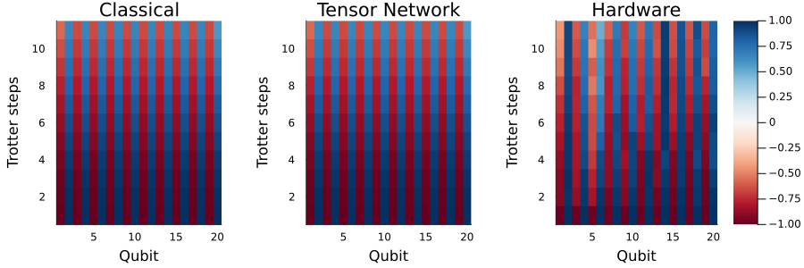
Daripada sampel bitstring yang diperoleh daripada perkakasan kuantum, kita kira kemagnetan bagi setiap tapak (nilai jangkaan $\langle Z\rangle$ qubit tunggal) dengan memurnikan $(-1)^{b_i}$ ke atas semua shot, dengan $b_i$ ialah bit yang diukur bagi qubit $i$ . Kemudian kita plotkan kemagnetan sebagai peta haba merentas qubit dan langkah Trotter, membandingkan tiga kaedah secara berdampingan: simulasi klasik tepat, simulasi rangkaian tensor tanpa hingar, dan pelaksanaan pada perkakasan.

# Compute expectation values
# 0 -> 1, 1 -> -1
z_expval(samples, i) = mean((-1)^s[i] for s in samples)

magnetizations = [z_expval(all_samples[i], q) for i in 1:length(all_samples), q in 1:N]

11×20 Matrix{Float64}:
 -0.996094  0.998047  -0.990234  0.998047  …  1.0       -0.988281  0.994141
 -0.925781  0.980469  -0.878906  0.96875      0.970703  -0.976562  0.988281
 -0.916016  0.992188  -0.837891  0.957031     0.962891  -0.966797  0.953125
 -0.884766  0.970703  -0.824219  0.90625      0.908203  -0.939453  0.892578
 -0.835938  0.96875   -0.814453  0.884766     0.931641  -0.902344  0.908203
 -0.777344  0.958984  -0.78125   0.871094  …  0.935547  -0.876953  0.939453
 -0.732422  0.933594  -0.767578  0.8125       0.884766  -0.835938  0.890625
 -0.650391  0.916016  -0.771484  0.771484     0.853516  -0.773438  0.837891
 -0.537109  0.902344  -0.705078  0.742188     0.875     -0.662109  0.833984
 -0.472656  0.923828  -0.652344  0.728516     0.839844  -0.695312  0.808594
 -0.4375    0.923828  -0.613281  0.681641  …  0.890625  -0.658203  0.8125

Tiga panel di bawah menunjukkan kemagnetan tapak $\langle Z_i \rangle$ sebagai fungsi indeks qubit (paksi-x) dan langkah Trotter (paksi-y). Pada $\delta t = 0.05$ dengan $r_{\max} = 10$ , jumlah masa evolusi ialah $\tau = r_{\max} \cdot \delta t = 0.5$ , yang cukup singkat sehingga corak antiferomagnet awal belum mereput — ketiga-tiga kaedah menunjukkan corak berselang-seli yang kuat. Hasil klasik dan rangkaian tensor kini sangat sepadan, mengesahkan bahawa ralat Trotter kecil pada saiz langkah ini. Hasil perkakasan secara umumnya mengikut dua yang lain, walaupun sesetengah qubit menyimpang daripada simulasi lebih daripada yang lain, mencerminkan variasi kualiti qubit merentas backend. Sisihan ini bertambah pada langkah Trotter yang lebih lewat apabila kedalaman Circuit meningkat.

# plot magnetization as a function of time
l = @layout [a{0.3w} b{0.3w} c{0.44w}]
plot(
    heatmap(classical_magnetizations, title="Classical", clims=(-1,1), color=:RdBu,
        xlabel="Qubit", ylabel="Trotter steps", colorbar=false),
    heatmap(tn_magnetizations, title="Tensor Network", clims=(-1,1), color=:RdBu,
        xlabel="Qubit", ylabel="Trotter steps", colorbar=false),
    heatmap(magnetizations, title="Hardware", clims=(-1,1), color=:RdBu,
        xlabel="Qubit", ylabel="Trotter steps", colorbar=true),
    layout=l, size=(900,300),
    bottom_margin=5mm, left_margin=5mm, right_margin=6mm
)

Output of the previous code cell

Contoh perkakasan berskala besar

Langkah 1–4 dalam satu aliran kerja

Sekarang kita gabungkan keempat-empat langkah di atas menjadi satu aliran kerja, pada skala yang melangkaui kemampuan simulasi klasik tepat. Daripada menyelesaikan kemagnetan tapak demi tapak, kita jejaki satu ukuran skalar bagi tertib antiferomagnet, iaitu kemagnetan berselang-seli (staggered magnetization):

\langle M_s \rangle = \frac{1}{N} \sum_{i=1}^{N} (-1)^i \langle Z_i \rangle

Tanda berselang-seli dalam penjumlahan menjadikan isyarat kelihatan. Bagi keadaan awal Néel $|0101\ldots01\rangle$ , setiap sebutan menyumbang $+1$ , jadi $\langle M_s\rangle = 1$ , manakala purata biasa $\frac{1}{N}\sum_i \langle Z_i\rangle$ lenyap sepenuhnya untuk semua $t$ . Apabila medan melintang mengacau corak berselang-seli, $\langle M_s\rangle$ mereput ke arah $0$ , jadi kemagnetan berselang-seli memberitahu kita berapa banyak tertib awal yang kekal semasa evolusi masa.

Kita juga menggunakan contoh ini untuk melihat bagaimana saiz langkah Trotter mempengaruhi ketepatan. Kita tetapkan jumlah masa evolusi $T = 1.5$ dan ubah bilangan langkah Trotter $r \in \{3, 6, 12\}$ , supaya $\delta t = T/r$ . Pada perkakasan, dua punca ralat bersaing: $\delta t$ yang lebih kecil mengurangkan ralat Trotter, tetapi memerlukan gate dua qubit yang berkadar lebih banyak, yang mengumpul lebih banyak hingar perkakasan.

# -------------------------Step 1-------------------------
# Map classical inputs to a quantum problem.
N_large = 100
g_large = named_grid((N_large,))
h_large = fill(1.0, N_large)       # transverse field on every site
J_large = fill(1.0, N_large - 1)   # nearest-neighbor ZZ couplings on the chain

T_total = 1.5                    # fixed total evolution time
r_list = [3, 6, 12]       # varying Trotter steps; δt = T_total/r
sweep = [(r, k) for r in r_list for k in 0:r]

qc_list_large = [make_trotter_circuit(h_large, J_large, N_large, T_total/r, k)
                 for (r, k) in sweep]

# -------------------------Step 2-------------------------
# Optimize the problem for quantum hardware execution.
tqc_list_large = [transpile(qc, target)[1] for qc in qc_list_large]
# Print the 2q gate count and depth of the deepest circuit at each δt",
for r in r_list
    i = findfirst(==((r, r)), sweep)   # the k = r circuit reaches the full T_total
    println("  δt = $(round(T_total/r, digits=4))  →  $(r+1) time points, ",
        "deepest circuit = $(r) Trotter steps, ",
        "2q count = $(two_qubit_count(tqc_list_large[i])), ",
        "2q depth = $(two_qubit_depth(tqc_list_large[i]))")
end

# -------------------------Step 3-------------------------
# Execute using Qiskit primitives.
shots_large = 4096

job_list_large = [run_sampler_job(service, backend, tqc, shots_large)
                  for tqc in tqc_list_large]

δt = 0.5  →  4 time points, deepest circuit = 3 Trotter steps, 2q count = 594, 2q depth = 206
  δt = 0.25  →  7 time points, deepest circuit = 6 Trotter steps, 2q count = 1188, 2q depth = 218
  δt = 0.125  →  13 time points, deepest circuit = 12 Trotter steps, 2q count = 2376, 2q depth = 242

24-element Vector{QiskitIBMRuntime.Job}:
 QiskitIBMRuntime.Job(Ptr{QiskitIBMRuntime.LibQiskitIBMRuntime.Job} @0x0000000104c1a750)
 QiskitIBMRuntime.Job(Ptr{QiskitIBMRuntime.LibQiskitIBMRuntime.Job} @0x0000000102e0a270)
 QiskitIBMRuntime.Job(Ptr{QiskitIBMRuntime.LibQiskitIBMRuntime.Job} @0x0000000104c21a50)
 QiskitIBMRuntime.Job(Ptr{QiskitIBMRuntime.LibQiskitIBMRuntime.Job} @0x0000000102e05120)
 QiskitIBMRuntime.Job(Ptr{QiskitIBMRuntime.LibQiskitIBMRuntime.Job} @0x0000000104c2a6e0)
 QiskitIBMRuntime.Job(Ptr{QiskitIBMRuntime.LibQiskitIBMRuntime.Job} @0x0000000102e0d140)
 QiskitIBMRuntime.Job(Ptr{QiskitIBMRuntime.LibQiskitIBMRuntime.Job} @0x0000000102e0b640)
 QiskitIBMRuntime.Job(Ptr{QiskitIBMRuntime.LibQiskitIBMRuntime.Job} @0x0000000104c1a200)
 QiskitIBMRuntime.Job(Ptr{QiskitIBMRuntime.LibQiskitIBMRuntime.Job} @0x00000004b312eb90)
 QiskitIBMRuntime.Job(Ptr{QiskitIBMRuntime.LibQiskitIBMRuntime.Job} @0x0000000104c22060)
 QiskitIBMRuntime.Job(Ptr{QiskitIBMRuntime.LibQiskitIBMRuntime.Job} @0x00000004b31ea4e0)
 QiskitIBMRuntime.Job(Ptr{QiskitIBMRuntime.LibQiskitIBMRuntime.Job} @0x0000000104c1ccf0)
 QiskitIBMRuntime.Job(Ptr{QiskitIBMRuntime.LibQiskitIBMRuntime.Job} @0x0000000104c2af50)
 QiskitIBMRuntime.Job(Ptr{QiskitIBMRuntime.LibQiskitIBMRuntime.Job} @0x00000004b312ffb0)
 QiskitIBMRuntime.Job(Ptr{QiskitIBMRuntime.LibQiskitIBMRuntime.Job} @0x00000004b0e89700)
 QiskitIBMRuntime.Job(Ptr{QiskitIBMRuntime.LibQiskitIBMRuntime.Job} @0x0000000102e15070)
 QiskitIBMRuntime.Job(Ptr{QiskitIBMRuntime.LibQiskitIBMRuntime.Job} @0x0000000102e10d40)
 QiskitIBMRuntime.Job(Ptr{QiskitIBMRuntime.LibQiskitIBMRuntime.Job} @0x00000004af5a5d10)
 QiskitIBMRuntime.Job(Ptr{QiskitIBMRuntime.LibQiskitIBMRuntime.Job} @0x0000000102e12500)
 QiskitIBMRuntime.Job(Ptr{QiskitIBMRuntime.LibQiskitIBMRuntime.Job} @0x0000000102e14870)
 QiskitIBMRuntime.Job(Ptr{QiskitIBMRuntime.LibQiskitIBMRuntime.Job} @0x0000000102e10730)
 QiskitIBMRuntime.Job(Ptr{QiskitIBMRuntime.LibQiskitIBMRuntime.Job} @0x00000004b237ca60)
 QiskitIBMRuntime.Job(Ptr{QiskitIBMRuntime.LibQiskitIBMRuntime.Job} @0x00000004b2c713a0)
 QiskitIBMRuntime.Job(Ptr{QiskitIBMRuntime.LibQiskitIBMRuntime.Job} @0x0000000102e13e90)

# Run this cell to check the job status
# Run the following cell for post-processing after all jobs complete
for (i, job) in enumerate(job_list_large)
    r, k = sweep[i]
    println("Job $i (δt=$(round(T_total/r, digits=4)), k=$k): ",
            get_job_status(job, service))
end

Job 1 (δt=0.5, k=0): Completed
Job 2 (δt=0.5, k=1): Completed
Job 3 (δt=0.5, k=2): Completed
Job 4 (δt=0.5, k=3): Completed
Job 5 (δt=0.25, k=0): Completed
Job 6 (δt=0.25, k=1): Completed
Job 7 (δt=0.25, k=2): Completed
Job 8 (δt=0.25, k=3): Completed
Job 9 (δt=0.25, k=4): Completed
Job 10 (δt=0.25, k=5): Completed
Job 11 (δt=0.25, k=6): Completed
Job 12 (δt=0.125, k=0): Completed
Job 13 (δt=0.125, k=1): Completed
Job 14 (δt=0.125, k=2): Completed
Job 15 (δt=0.125, k=3): Completed
Job 16 (δt=0.125, k=4): Completed
Job 17 (δt=0.125, k=5): Completed
Job 18 (δt=0.125, k=6): Completed
Job 19 (δt=0.125, k=7): Completed
Job 20 (δt=0.125, k=8): Completed
Job 21 (δt=0.125, k=9): Completed
Job 22 (δt=0.125, k=10): Completed
Job 23 (δt=0.125, k=11): Completed
Job 24 (δt=0.125, k=12): Completed

# -------------------------Step 4-------------------------
# Post-process and return the result in the desired classical format.
# Run this cell after all jobs are completed

# ⟨M_s⟩ = (1/N) Σ (-1)^i ⟨Z_i⟩, averaged over hardware shots
function staggered_magnetization(samples::AbstractVector{<:AbstractVector}, n::Int)
    s = 0.0
    for sample in samples
        s += sum((-1)^i * (1 - 2 * sample[i]) for i in 1:n) / n
    end
    return s / length(samples)
end

all_samples_large = [get_sampler_job_results(job, service) for job in job_list_large]
mags_hardware = [staggered_magnetization(s, N_large) for s in all_samples_large]

24-element Vector{Float64}:
9880371093750097
697231445312484
44886718750000276
29333496093750067
9882324218750095
8109619140625324
6457958984374791
4808593749999992
36695312500000055
2963671875000012
23831542968750055
9884472656250093
8566455078125492
7951171875000282
7050732421874865
610673828124981
529980468749995
4656054687500018
4149316406250024
3799462890625011
35178710937500185
3185888671875003
31287597656250016
29621093750000077

Pada $N=100$ , penyelesaian tepat daripada penyelesai ODE yang digunakan di atas tidak tercapai, kerana vektor keadaan sahaja memerlukan $2^{100} \approx 10^{30}$ amplitud. Sebaliknya kita menggunakan simulasi rangkaian tensor tanpa hingar bagi rantai 1D yang sama dengan langkah Trotter yang jauh lebih halus ( $r = 96$ , $\delta t \approx 0.016$ ) sebagai rujukan, yang ralat Trotter-nya boleh diabaikan berbanding mana-mana $\delta t$ yang kita jalankan pada perkakasan. Rujukan ini sendiri adalah hampiran: ralat utamanya kini ialah pemangkasan dimensi ikatan yang dibincangkan di atas, dilaporkan sebagai fidelity pemangkasan bagi setiap larian.

apply_kwargs = (; maxdim=64, cutoff=1e-10, normalize_tensors=true)

# Calculate the staggered magnetization given a tensor network state
staggered_magnetization(ψ_bpc::BeliefPropagationCache, n::Int) =
    sum((-1)^q * m for (q, m) in enumerate(z_expvals_from_tn_state(ψ_bpc, n))) / n

# Evolve a TN state and record the staggered magnetization at each step.
function compute_staggered_magnetization_tn(δt::Real, nsteps::Int; record_every::Int = 1)
    init_gates = neel_state_gates(N_large)
    step_gates = trotter_step_gates(h_large, J_large, N_large, δt)

    ψ_bpc, fid = apply_gates_to_tn_state(init_gates, tn_initial_state(g_large); apply_kwargs)
    times = [0.0]
    mags = [staggered_magnetization(ψ_bpc, N_large)]
    for k in 1:nsteps
        ψ_bpc, fid_step = apply_gates_to_tn_state(step_gates, ψ_bpc; apply_kwargs)
        fid *= fid_step
        if k % record_every == 0
            push!(times, k * δt)
            push!(mags, staggered_magnetization(ψ_bpc, N_large))
        end
    end
    println("  δt=$(round(δt, digits=5)), $(nsteps) steps: truncation fidelity ≈ $(round(fid, digits=5))")
    (times, mags)
end

# If the fidelity drifts from 1, raise `maxdim` in `apply_kwargs`.
# Under current setting, the tensor network simulation takes ~ 3 minutes on a laptop.
println("Tensor-network reference:")
r_ref = 96
times_ref, mags_ref = compute_staggered_magnetization_tn(T_total / r_ref, r_ref; record_every = r_ref ÷ 12)

Tensor-network reference:
  δt=0.01562, 96 steps: truncation fidelity ≈ 1.0

([0.0, 0.125, 0.25, 0.375, 0.5, 0.625, 0.75, 0.875, 1.0, 1.125, 1.25, 1.375, 1.5], Float32[1.0, 0.9695576, 0.8870231, 0.77430177, 0.6560442, 0.5499543, 0.46285573, 0.39298016, 0.33518773, 0.28527063, 0.24147007, 0.20369667, 0.17206171])

Plot di bawah menunjukkan kemagnetan berselang-seli sepanjang masa bagi tiga saiz langkah Trotter, berbanding rujukan rangkaian tensor tanpa hingar (hitam putus-putus).

plt = plot(xlabel = "Time", ylabel = "Staggered magnetization",
    title = "N = $(N_large) on $(backend.name), T = $(T_total)",
    legend = :topright, ylims = (-0.05, 1.05), size = (820, 480),
    bottom_margin = 5mm, left_margin = 5mm)

# Plot tensor network reference
plot!(plt, times_ref, mags_ref, lw = 2, ls = :dash, color = :black,
      label = "tensor network, δt → 0")

# Plot hardware result per Trotter step size
for (r, stop) in zip(r_list, cumsum(r_list .+ 1))
    plot!(plt, range(0, T_total, length = r + 1), mags_hardware[(stop - r):stop],
          marker = :circle, markersize = 4, lw = 2,
          label = "hardware, δt = $(round(T_total / r, digits = 4))")
end
plt

Output of the previous code cell

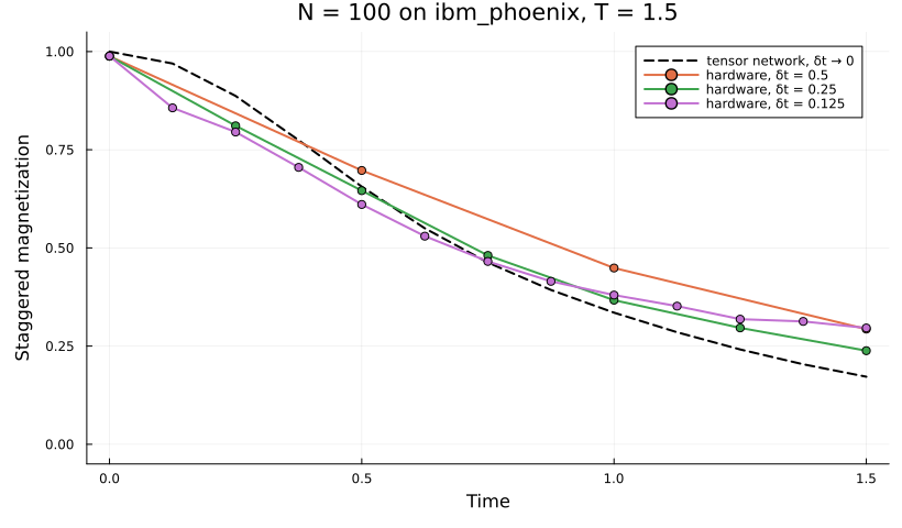
Secara keseluruhan, langkah Trotter paling kasar $\delta t = 0.5$ (titik oren) menunjukkan sisihan terbesar daripada rujukan rangkaian tensor, mungkin dengan sumbangan besar daripada ralat Trotter. Pada langkah yang lebih halus $\delta t = 0.25$ (titik hijau), hasil perkakasan lebih rapat dengan rujukan. Pada langkah paling halus $\delta t = 0.125$ (titik ungu), ralat Trotter paling kecil, namun persetujuannya lebih buruk berbanding pada $\delta t = 0.25$ . Dengan separuh saiz langkah, setiap titik masa memerlukan dua kali ganda gate dua qubit, dan hingar tambahan mengatasi pengurangan ralat Trotter. Oleh itu, memilih $\delta t$ untuk Circuit yang di-Trotter-kan pada perkakasan ialah pertukaran antara ralat Trotter dan hingar yang terkumpul daripada gate tambahan.

Langkah seterusnya

Anda mungkin berminat dengan bahan berikut:

Hasil pembelajaran​

Prasyarat​

Latar belakang​

Keperluan​

Persediaan​

Contoh simulator berskala kecil​

Penyelesaian tepat​

Simulasi berskala kecil bagi Circuit yang di-Trotter-kan​

Langkah 1: Petakan input klasik kepada masalah kuantum​

Langkah 2: Optimumkan masalah untuk pelaksanaan pada perkakasan kuantum​

Langkah 3: Laksanakan menggunakan primitif Qiskit​

Langkah 4: Pasca-proses dan pulangkan hasil dalam format klasik yang dikehendaki​

Contoh perkakasan berskala besar​

Langkah 1–4 dalam satu aliran kerja​

Langkah seterusnya​