Warm-start QAOA dengan Optimization Mapper Qiskit addon

Anggaran penggunaan: 9 minit pada Heron r3 (NOTA: Ini hanyalah anggaran. Masa larian anda mungkin berbeza.)

Hasil pembelajaran

Cara memetakan masalah max-cut kepada formulasi Quadratic Unconstrained Binary Optimization (QUBO) kuantum menggunakan qiskit-addon-opt-mapper
Cara melaksanakan dan menjalankan QAOA standard pada simulator
Cara menerapkan WS-QAOA dengan mengira relaksasi program kuadratik (QP) dan membina litar warm-start
Cara membandingkan penumpuan tenaga dan kualiti penyelesaian antara QAOA standard dan WS-QAOA

Prasyarat

Latar belakang

Quantum Approximate Optimization Algorithm (QAOA) adalah algoritma hibrid kuantum-klasik yang direka untuk menyelesaikan masalah optimumasi kombinatorial seperti max-cut dan formulasi QUBO am. Untuk pengenalan asas kepada QAOA dalam Qiskit, lihat tutorial QAOA; untuk teknik pembinaan litar yang lebih lanjut, lihat tutorial QAOA lanjutan.

Dalam QAOA standard:

Keadaan awal adalah superposisi seragam $|+\rangle^{\otimes n}$ .
Parameter berubah-ubah dimulakan secara rawak.
Pengoptimum klasik mencari parameter yang meminimumkan fungsi kos.

Walau bagaimanapun, untuk saiz masalah praktikal dan perkakasan kuantum berhingar, permulaan rawak boleh membawa kepada penumpuan yang perlahan, minimum tempatan yang lemah, dan kos optimumasi yang meningkat.

Warm-start QAOA (WS-QAOA) memperbaiki ini dengan menggabungkan wawasan optimumasi klasik secara terus ke dalam litar kuantum. Tutorial ini mengikuti kaedah yang diperkenalkan oleh Egger, Mareček, dan Woerner dalam Warm-starting quantum optimization. Idea utamanya adalah untuk:

Selesaikan relaksasi berterusan bagi masalah binari asal (program kuadratik ke atas $[0,1]^n$ bukannya $\{0,1\}^n$ ).
Kodkan penyelesaian relaksasi $c^*_i \in [0,1]$ ke dalam keadaan awal tersuai dengan menggunakan sudut putaran $Y$ $\theta_i = 2\arcsin(\sqrt{c^*_i})$ , supaya qubit $i$ bermula dalam keadaan yang kebarangkalian mengukur $|1\rangle$ ialah $c^*_i$ .
Gantikan mixer $X$ standard dengan mixer tersuai yang keadaan asasnya adalah keadaan awal warm-start, memastikan algoritma bermula berhampiran penyelesaian klasik dan boleh meneroka kawasan sekitarnya.

Parameter regularisasi $\varepsilon \in [0, 0.5]$ memotong $c^*_i$ menjauhi 0 dan 1 untuk mengelakkan isu kebolehcapaian; qubit yang dimulakan dalam $|0\rangle$ atau $|1\rangle$ tidak boleh digerakkan oleh Hamiltonian kos. Pada $\varepsilon = 0.5$ , WS-QAOA berkurangan secara tepat kepada QAOA standard.

Pemodelan masalah menggunakan pakej qiskit-addon-opt-mapper, yang kelas aplikasi Maxcut membina QUBO secara terus daripada graf, dan yang penukar serta penterjemahnya memetakan masalah yang terhasil kepada Hamiltonian kuantum.

Keperluan

Sebelum memulakan tutorial ini, pastikan anda telah memasang perkara berikut:

Qiskit SDK v2.0 atau lebih baru, dengan sokongan visualisasi
Qiskit Runtime v0.43 atau lebih baru (pip install qiskit-ibm-runtime)
Optimization Mapper Qiskit addon (pip install qiskit-addon-opt-mapper)
SciPy (pip install scipy)
NetworkX (pip install networkx)

Persediaan

Import semua pustaka yang diperlukan dan takrifkan fungsi pembantu yang digunakan di seluruh tutorial ini.

# Added by doQumentation — required packages for this notebook
!pip install -q matplotlib networkx numpy qiskit qiskit-addon-opt-mapper qiskit-ibm-runtime scipy

import numpy as np
import matplotlib.pyplot as plt
import networkx as nx
from scipy.optimize import minimize

from qiskit.circuit import QuantumCircuit, ParameterVector
from qiskit.circuit.library import qaoa_ansatz
from qiskit.quantum_info import Statevector
from qiskit.primitives import StatevectorEstimator, StatevectorSampler
from qiskit.transpiler.preset_passmanagers import generate_preset_pass_manager
from qiskit_ibm_runtime import (
    QiskitRuntimeService,
    Session,
    EstimatorOptions,
    EstimatorV2 as Estimator,
    SamplerV2 as Sampler,
)

from qiskit_addon_opt_mapper.applications import Maxcut
from qiskit_addon_opt_mapper.converters import OptimizationProblemToQubo
from qiskit_addon_opt_mapper.translators import to_ising

Contoh simulator berskala kecil

Kami menggunakan masalah max-cut kecil pada graf berpemberat sebagai contoh berjalan kami. Max-cut bertanya: diberi graf $G=(V,E)$ dengan pemberat tepi $w_{ij}$ , cari sekatan bucu kepada dua set $S$ dan $\bar{S}$ yang memaksimumkan jumlah pemberat tepi yang melintasi potongan.

Sebagai masalah minimumasi QUBO, max-cut boleh ditulis sebagai: $\min_{x \in \{0,1\}^n} -\sum_{(i,j) \in E} w_{ij}(x_i + x_j - 2x_i x_j)$

Kami bekerja dengan graf empat-nod untuk kebolehurusan pada simulator.

Langkah 1: Petakan input klasik kepada masalah kuantum

Kami mentakrifkan masalah max-cut menggunakan kelas aplikasi Maxcut daripada qiskit-addon-opt-mapper, yang membina formulasi QUBO secara terus daripada graf. Kami kemudian menukarnya kepada QUBO dan menterjemahkannya kepada Hamiltonian Ising (SparsePauliOp) yang sesuai untuk QAOA. Kami juga menyelesaikan relaksasi berterusan bagi QUBO — menggantikan kekangan binari $x_i \in \{0,1\}$ dengan $x_i \in [0,1]$ — untuk mendapatkan titik awal warm-start $c^*$ .

# Define a 4-node weighted graph for the max-cut problem
n_nodes = 4
edges = [(0, 1, 1.0), (0, 2, 1.0), (1, 2, 1.0), (1, 3, 1.0), (2, 3, 1.0)]

G = nx.Graph()
G.add_nodes_from(range(n_nodes))
G.add_weighted_edges_from(edges)

pos = nx.spring_layout(G, seed=42)
edge_labels = {(u, v): d["weight"] for u, v, d in G.edges(data=True)}

fig, ax = plt.subplots(figsize=(4, 3))
nx.draw(G, pos, with_labels=True, node_color="lightblue", ax=ax)
nx.draw_networkx_edge_labels(G, pos, edge_labels=edge_labels, ax=ax)
ax.set_title("Max-Cut graph")
plt.tight_layout()
plt.show()

Output of the previous code cell

Graf ini mempunyai lima tepi. Max-cut optimum membahagikan nod kepada $S = \{0, 3\}$ dan $\bar{S} = \{1, 2\}$ (atau pelengkapnya), memotong empat daripada lima tepi untuk nilai potongan 4.

# Build the max-cut problem directly from the NetworkX graph using the
# Maxcut application class. Internally it constructs the QUBO
#   minimize  -sum_{(i,j) in E} w_ij * (x_i + x_j - 2*x_i*x_j)
# (each edge contributes -w to the linear terms and +2w to the quadratic
# term), so we get the same OptimizationProblem without the boilerplate.
maxcut = Maxcut(G)
prob = maxcut.to_optimization_problem()
print(prob.prettyprint())

Problem name: Max-cut

Maximize
  -2*x_0*x_1 - 2*x_0*x_2 - 2*x_1*x_2 - 2*x_1*x_3 - 2*x_2*x_3 + 2*x_0 + 3*x_1
  + 3*x_2 + 2*x_3

Subject to
  No constraints

  Binary variables (4)
    x_0 x_1 x_2 x_3

Kelas Maxcut membungkus pembinaan QUBO supaya kami tidak perlu mengembangkan objektif max-cut secara manual. Objektif yang dicetak menunjukkan pekali linear setiap pembolehubah (berapa banyak ia menyumbang secara individu kepada potongan) dan pekali kuadratik setiap terma silang (penalti kerana meletakkan dua nod bersebelahan pada sisi yang sama). OptimizationProblem yang mendasari yang dikembalikan oleh to_optimization_problem() menyokong pembolehubah binari, integer, berterusan, dan spin, dan merupakan objek yang sama yang dijangkakan oleh penukar dan penterjemah yang digunakan dalam langkah seterusnya.

# Convert the OptimizationProblem to a QUBO, then translate to an Ising Hamiltonian
#
# The substitution x_i = (1 - z_i)/2  maps binary variables to spin operators,
# yielding a Hamiltonian H_C = sum_i h_i Z_i + sum_{i<j} J_ij Z_i Z_j + constant.
# QAOA minimizes <H_C> to find the ground state, which encodes the optimal cut.
converter = OptimizationProblemToQubo()
qubo = converter.convert(prob)

cost_operator, offset = to_ising(qubo)
n_qubits = cost_operator.num_qubits

print(f"Cost Hamiltonian H_C ({n_qubits} qubits):")
print(cost_operator)
print(f"\nOffset (constant shift): {offset}")
print("  QUBO value = Ising energy + offset")

Cost Hamiltonian H_C (4 qubits):
SparsePauliOp(['IIZZ', 'IZIZ', 'IZZI', 'ZIZI', 'ZZII'],
              coeffs=[0.5+0.j, 0.5+0.j, 0.5+0.j, 0.5+0.j, 0.5+0.j])

Offset (constant shift): -2.5
  QUBO value = Ising energy + offset

Penterjemah to_ising mengembalikan SparsePauliOp yang mewakili $H_C$ dan offset skalar sedemikian rupa sehingga $\text{nilai QUBO} = \langle H_C \rangle + \text{offset}$ . Untuk masalah max-cut ini dengan semua pemberat unit, $h_i = 0$ untuk semua qubit (graf adalah simetri dalam terma linear selepas penggantian $x_i \to z_i$ ), dan setiap tepi menyumbang gandingan $Z_i Z_j$ dengan kekuatan $+0.5$ . Nilai eigen minimum $H_C$ sepadan dengan max-cut.

# Solve the continuous (QP) relaxation to obtain the warm-start point c*
#
# The QP relaxation replaces the binary constraint x_i in {0,1} with x_i in [0,1]
# and minimizes the same quadratic objective. Its solution c*_i gives the
# probability that variable i should be 1 according to the classical relaxation.
#
# The max-cut QUBO has a non-convex quadratic matrix (negative eigenvalues),
# so the relaxed problem has multiple local minima. A naive single start from
# [0.5,...,0.5] converges to the symmetric saddle point c* = [0.5,...,0.5],
# which carries no useful structural information about the problem.
# Multi-start optimization is used to reliably find the global minimum.
Q = qubo.objective.quadratic.to_array(symmetric=True)
mu = qubo.objective.linear.to_array()

def qp_objective(x_cont):
    """Continuous relaxation of the QUBO objective."""
    return x_cont @ Q @ x_cont + mu @ x_cont + qubo.objective.constant

bounds = [(0.0, 1.0)] * n_qubits

rng = np.random.default_rng(42)
best_val = np.inf
c_star = None
for _ in range(200):
    x0 = rng.uniform(0.0, 1.0, n_qubits)
    result = minimize(qp_objective, x0, method="L-BFGS-B", bounds=bounds)
    if result.fun < best_val:
        best_val = result.fun
        c_star = result.x

print(f"QP relaxation solution c* = {np.round(c_star, 4)}")
print(f"QP objective value        = {best_val:.4f}")

QP relaxation solution c* = [1. 0. 0. 1.]
QP objective value        = -4.0000

Penyelesai multi-start menemui $c^* = [1, 0, 0, 1]$ (atau pelengkapnya $[0, 1, 1, 0]$ ), iaitu penyelesaian binari optimum yang sebenar. Untuk masalah ini relaksasi QP adalah ketat, minimum berterusan bertepatan dengan optimum integer, bermakna relaksasi segera mengenal pasti potongan terbaik. Selepas regularisasi dengan $\varepsilon = 0.25$ dalam Langkah 2, penyelesaian ini akan dikodkan ke dalam keadaan awal warm-start.

Langkah 2: Optimumkan masalah untuk pelaksanaan perkakasan kuantum

Kami membina dua litar QAOA dan menyediakan sudut warm-start daripada penyelesaian QP.

QAOA standard menggunakan superposisi seragam $|+\rangle^{\otimes n}$ sebagai keadaan awal dan mixer $X$ standard $H_M = -\sum_i X_i$ , dilaksanakan sebagai $\prod_i R_X(-2\beta)$ setiap lapisan.

Warm-start QAOA (WS-QAOA) daripada [1] membuat dua perubahan struktur setiap qubit $i$ :

Keadaan awal: $R_Y(\theta_i)|0\rangle$ dengan $\theta_i = 2\arcsin(\sqrt{c^*_i})$ , supaya kebarangkalian mengukur $|1\rangle$ bersamaan dengan $c^*_i$ .
Mixer tersuai: $R_Y(\theta_i)\, R_Z(-2\beta)\, R_Y(-\theta_i)$ , yang mempunyai $R_Y(\theta_i)|0\rangle$ sebagai keadaan asasnya. Ini bermakna WS-QAOA bermula dalam keadaan asas mixernya sendiri, sifat yang sama yang dipenuhi oleh QAOA standard dengan $|+\rangle$ dan mixer $X$ .

Nota mengenai lapisan: Pada p=1 (satu lapisan QAOA tunggal), QAOA standard terhad secara analitikal kepada ~49% tenaga optimum pada graf yang mengandungi segitiga (graf ini mempunyai segitiga 0-1-2). Warm start memintas had ini dengan mengkodkan pengetahuan sedia ada tentang penyelesaian secara terus ke dalam keadaan awal.

# Number of QAOA layers (each layer = one cost unitary + one mixer unitary)
p = 1

# Regularization: clip c* to [epsilon, 1-epsilon] so no qubit is initialized
# in |0> or |1>, which would freeze it under the cost Hamiltonian.
epsilon = 0.25

c_clipped = np.clip(c_star, epsilon, 1 - epsilon)
thetas = 2 * np.arcsin(np.sqrt(c_clipped))

print(f"Continuous relaxation c*  = {np.round(c_star, 4)}")
print(f"After regularization      = {np.round(c_clipped, 4)}")
print(f"Warm-start angles theta   = {np.round(thetas, 4)} radians")
print()
print("Angle interpretation:")
print("  theta = 0      <->  c* = 0   (qubit points toward |0>)")
print(
    "  theta = pi/2   <->  c* = 0.5 (qubit in equal superposition, like |+>)"
)
print("  theta = pi     <->  c* = 1   (qubit points toward |1>)")

Continuous relaxation c*  = [1. 0. 0. 1.]
After regularization      = [0.75 0.25 0.25 0.75]
Warm-start angles theta   = [2.0944 1.0472 1.0472 2.0944] radians

Angle interpretation:
  theta = 0      <->  c* = 0   (qubit points toward |0>)
  theta = pi/2   <->  c* = 0.5 (qubit in equal superposition, like |+>)
  theta = pi     <->  c* = 1   (qubit points toward |1>)

Selepas pemotongan, $c^* = 1$ menjadi $1 - \varepsilon = 0.75$ dan $c^* = 0$ menjadi $\varepsilon = 0.25$ . Sudut yang terhasil $\theta \approx [2.09, 1.05, 1.05, 2.09]$ radian memutarkan qubit 0 dan 3 kuat ke arah $|1\rangle$ dan qubit 1 dan 2 ke arah $|0\rangle$ , secara terus mengkodkan struktur potongan optimum ke dalam keadaan kuantum awal.

def apply_cost_unitary(qc, cost_op, gamma):
    """Apply exp(-i * gamma * H_C) to the circuit.

    Each Pauli term in H_C contributes a rotation gate:
      - Single-Z term h_i * Z_i  ->  RZ(2 * gamma * h_i) on qubit i
      - Two-Z term J_ij * Z_i Z_j  ->  CNOT, RZ(2 * gamma * J_ij), CNOT
    """
    for pauli_term, coeff in zip(cost_op.paulis, cost_op.coeffs):
        indices = [
            j for j, q in enumerate(pauli_term.to_label()[::-1]) if q == "Z"
        ]
        if len(indices) == 1:
            qc.rz(2 * gamma * coeff.real, indices[0])
        elif len(indices) == 2:
            qc.cx(indices[0], indices[1])
            qc.rz(2 * gamma * coeff.real, indices[1])
            qc.cx(indices[0], indices[1])

def build_ws_qaoa(cost_op, n_layers, n_qubits, thetas):
    """WS-QAOA: warm-start initial state + custom per-qubit mixer.

    Per Egger et al. (2021) Eq. (1)-(2):
      Initial state per qubit i:  R_Y(theta_i) |0>
      Mixer gate per qubit i:     R_Y(theta_i) R_Z(-2*beta) R_Y(-theta_i)
    """
    gammas = ParameterVector("γ", n_layers)
    betas = ParameterVector("β", n_layers)
    qc = QuantumCircuit(n_qubits)
    for i, theta in enumerate(thetas):
        qc.ry(theta, i)  # warm-start initial state
    for k in range(n_layers):
        apply_cost_unitary(qc, cost_op, gammas[k])
        for i, theta in enumerate(thetas):
            qc.ry(theta, i)
            qc.rz(-2 * betas[k], i)
            qc.ry(-theta, i)
    return qc, gammas, betas

# Standard QAOA via the Qiskit built-in helper:
# qaoa_ansatz prepares |+>^n, then alternates exp(-i*gamma*H_C) with the
# default X-mixer for `reps` layers. The returned circuit exposes the
# variational parameters via std_qc.parameters.
std_qc = qaoa_ansatz(cost_operator, reps=p)

# WS-QAOA: keep the custom builder. The per-qubit mixer
# R_Y(theta_i) R_Z(-2*beta) R_Y(-theta_i) is implemented as an explicit gate
# sequence rather than as a SparsePauliOp, so we construct the circuit
# directly to stay close to the Egger et al. (2021) formulation.
ws_qc, ws_gammas, ws_betas = build_ws_qaoa(cost_operator, p, n_qubits, thetas)

Untuk ansatz standard kami mendelegasikan kepada qaoa_ansatz, yang membina $|+\rangle^{\otimes n}$ , mengaplikasikan unitari kos, dan mengaplikasikan mixer $X$ lalai untuk setiap lapisan reps. Untuk WS-QAOA kami mengekalkan pembantu eksplisit build_ws_qaoa kerana mixer setiap qubit $R_Y(\theta)\,R_Z(-2\beta)\,R_Y(-\theta)$ dinyatakan sebagai urutan get bukannya sebagai jumlah Pauli. Pembantu apply_cost_unitary membaca terus daripada Hamiltonian SparsePauliOp, jadi ia mengendalikan mana-mana masalah QUBO tanpa pembinaan litar secara manual.

print("Standard QAOA circuit (p=1):")
std_qc.draw("mpl", fold=-1)

Standard QAOA circuit (p=1):

Output of the previous code cell

print("\nWS-QAOA circuit (p=1):")
ws_qc.draw("mpl", fold=-1)

WS-QAOA circuit (p=1):

Output of the previous code cell

Kedua-dua litar mengikuti struktur yang sama: lapisan penyediaan keadaan awal, kemudian $p$ lapisan unitari-kos dan unitari-mixer berselang-seli. Dalam litar WS-QAOA, get $R_Y$ pembukaan mengkodkan $c^*$ , dan mixer menggantikan setiap $R_X$ dengan triplet $R_Y$ – $R_Z$ – $R_Y$ terkonjugasi. Perbezaan kedalaman litar antara kedua-duanya berkembang secara linear dengan $p$ , tetapi kekal boleh diurus pada kedalaman rendah.

Langkah 3: Laksanakan menggunakan primitif Qiskit

Kami menggunakan StatevectorEstimator untuk simulasi tepat, bebas hingar. Fungsi minimize daripada SciPy dengan pengoptimum COBYLA memacu gelung berubah-ubah, memanggil estimator pada setiap iterasi untuk menilai $\langle H_C \rangle$ bagi set parameter tertentu $(\gamma, \beta)$ .

Kedua-dua algoritma menggunakan parameter awal yang berbeza yang mencerminkan apa yang diketahui oleh setiap satu sebelum optimumasi:

QAOA standard: Permulaan rawak dalam $[0, \pi]$ — sesuai kerana tiada maklumat struktur tersedia.
WS-QAOA: $\gamma = 0$ , $\beta = \pi/4$ — pada $\gamma=0$ unitari kos adalah identiti, jadi penilaian litar pertama sekali mensampel terus daripada keadaan awal warm-start. Ini memberikan COBYLA isyarat permulaan yang kuat yang selari dengan penyelesaian klasik.

estimator = StatevectorEstimator()

def make_cost_fn(circuit, param_order, cost_op, estimator, history):
    """Return a scalar cost function compatible with scipy.optimize.minimize."""

    def cost_fn(params):
        bound = circuit.assign_parameters(dict(zip(param_order, params)))
        job = estimator.run([(bound, cost_op)])
        energy = job.result()[0].data.evs.real
        history.append(energy)
        return energy

    return cost_fn

# Standard QAOA: random initialization
np.random.seed(42)
std_param_order = list(std_qc.parameters)
std_params0 = np.random.uniform(0, np.pi, len(std_param_order))
std_history = []

std_result = minimize(
    make_cost_fn(
        std_qc, std_param_order, cost_operator, estimator, std_history
    ),
    std_params0,
    method="COBYLA",
    options={"maxiter": 300, "rhobeg": 0.5},
)
print(f"Standard QAOA optimal energy : {std_result.fun:.4f}")
print(f"  optimal params: {std_result.x.round(4)}")
print(f"  optimizer calls: {len(std_history)}")

# WS-QAOA: informed initialization
ws_params0 = np.concatenate([np.zeros(p), np.full(p, np.pi / 4)])
ws_history = []
ws_param_order = list(ws_gammas) + list(ws_betas)

ws_result = minimize(
    make_cost_fn(ws_qc, ws_param_order, cost_operator, estimator, ws_history),
    ws_params0,
    method="COBYLA",
    options={"maxiter": 300, "rhobeg": 0.5},
)
print(f"\nWS-QAOA optimal energy       : {ws_result.fun:.4f}")
print(
    f"  optimal params: gamma={ws_result.x[:p].round(4)}, beta={ws_result.x[p:].round(4)}"
)
print(f"  optimizer calls: {len(ws_history)}")

Standard QAOA optimal energy : -0.5859
  optimal params: [0.6803 2.0533]
  optimizer calls: 47

WS-QAOA optimal energy       : -1.5000
  optimal params: gamma=[-0.0001], beta=[1.5708]
  optimizer calls: 42

Titik permulaan bermaklumat WS-QAOA bermakna COBYLA bermula dengan nilai tenaga yang bermakna berhampiran penyelesaian warm-start, sementara QAOA standard bermula daripada titik yang secara asasnya rawak pada landskap tenaga. Perbezaan kualiti permulaan ini adalah penggerak utama jurang penumpuan yang kelihatan dalam Langkah 4.

# Compute the exact optimal energy by brute-force over all 2^n bitstrings
all_energies = [
    Statevector.from_label(format(k, f"0{n_qubits}b"))
    .expectation_value(cost_operator)
    .real
    for k in range(2**n_qubits)
]
optimal_energy = min(all_energies)

print(f"Exact optimal energy         : {optimal_energy:.4f}")
print(f"Standard QAOA approx. ratio  : {std_result.fun / optimal_energy:.4f}")
print(f"WS-QAOA approx. ratio        : {ws_result.fun / optimal_energy:.4f}")

Exact optimal energy         : -1.5000
Standard QAOA approx. ratio  : 0.3906
WS-QAOA approx. ratio        : 1.0000

Nisbah penghampiran ditakrifkan sebagai $\langle H_C \rangle_{\text{QAOA}} / E_{\text{opt}}$ . Untuk masalah minimumasi di mana $E_{\text{opt}} < 0$ , nisbah yang lebih hampir kepada 1 bermakna algoritma menemui tenaga yang lebih rendah (penyelesaian yang lebih baik). Carian brute-force ke atas semua $2^n$ keadaan asas hanya boleh dilaksanakan untuk $n$ yang kecil dan berfungsi sebagai rujukan kebenaran asas.

Langkah 4: Pasca-proses dan kembalikan hasil dalam format klasik yang dikehendaki

Kami memvisualisasikan penumpuan, mensampel litar yang dioptimumkan untuk penyelesaian bitstring, mendekod bitstring tersebut kembali kepada sekatan max-cut, dan meringkaskan hasil akhir.

fig, ax = plt.subplots(figsize=(7, 4))
ax.plot(std_history, label="Standard QAOA", alpha=0.85)
ax.plot(ws_history, label="WS-QAOA", alpha=0.85)
ax.axhline(
    optimal_energy,
    color="k",
    linestyle="--",
    label=f"Exact optimal ({optimal_energy:.2f})",
)
ax.set_xlabel("Optimizer call")
ax.set_ylabel(r"$\langle H_C \rangle$")
ax.set_title("Convergence: Standard QAOA vs. WS-QAOA")
ax.legend()
plt.tight_layout()
plt.show()

Output of the previous code cell

Plot penumpuan menunjukkan tenaga $\langle H_C \rangle$ pada setiap penilaian fungsi COBYLA. QAOA standard pada $p=1$ terhad kepada ~49% tenaga optimum pada graf ini (maksimum teori untuk QAOA $p=1$ pada graf dengan segitiga), menetap sekitar $-0.74$ . WS-QAOA, dimulakan hampir dengan penyelesaian optimum, menumpu dengan cepat hampir kepada $-1.50$ (optimum tepat) dengan jauh lebih sedikit iterasi. Ini menunjukkan kelebihan utama warm start: pada kedalaman litar yang sama, ia mencapai penyelesaian yang jauh lebih baik.

# Sample the optimized circuits to recover the most probable bitstring solutions
sampler = StatevectorSampler()
shots = 1024

def get_best_bitstring(circuit, param_order, optimal_params, sampler, shots):
    bound = circuit.assign_parameters(dict(zip(param_order, optimal_params)))
    bound.measure_all()
    job = sampler.run([bound], shots=shots)
    counts = job.result()[0].data.meas.get_counts()
    return max(counts, key=counts.get), counts

def evaluate_cut(bitstring, G):
    """Compute the Max-Cut value for a bitstring node assignment."""
    x = [int(b) for b in bitstring]
    cut_val = sum(
        w for u, v, w in G.edges.data("weight", default=1) if x[u] != x[v]
    )
    set0 = [i for i, b in enumerate(bitstring) if b == "0"]
    set1 = [i for i, b in enumerate(bitstring) if b == "1"]
    return cut_val, set0, set1

# Qiskit bitstring ordering: rightmost character = qubit 0
def decode_bitstring(bs):
    return bs[::-1]

std_best, std_counts = get_best_bitstring(
    std_qc, std_param_order, std_result.x, sampler, shots
)
ws_best, ws_counts = get_best_bitstring(
    ws_qc, ws_param_order, ws_result.x, sampler, shots
)

std_cut, std_s0, std_s1 = evaluate_cut(decode_bitstring(std_best), G)
ws_cut, ws_s0, ws_s1 = evaluate_cut(decode_bitstring(ws_best), G)

print(f"Standard QAOA most-probable bitstring : {std_best}")
print(f"  Partition: S={std_s0}, S̄={std_s1}  |  cut value = {std_cut}")
print()
print(f"WS-QAOA most-probable bitstring       : {ws_best}")
print(f"  Partition: S={ws_s0}, S̄={ws_s1}  |  cut value = {ws_cut}")

Standard QAOA most-probable bitstring : 0110
  Partition: S=[0, 3], S̄=[1, 2]  |  cut value = 4.0

WS-QAOA most-probable bitstring       : 0110
  Partition: S=[0, 3], S̄=[1, 2]  |  cut value = 4.0

Bitstring daripada Sampler dikembalikan dengan qubit 0 pada kedudukan paling kanan, jadi membalikkan rentetan memetakan indeks $i$ kepada pembolehubah $x_i$ . Nilai potongan adalah jumlah pemberat tepi yang melintasi sekatan, iaitu apa yang disasarkan oleh masalah max-cut untuk dimaksimumkan. Nilai potongan 4 menggunakan empat daripada lima tepi yang tersedia, iaitu maksimum teori untuk graf ini.

# Visualize the WS-QAOA solution on the graph
fig, axes = plt.subplots(1, 2, figsize=(8, 3))

for ax, s0, s1, cut, title in [
    (axes[0], std_s0, std_s1, std_cut, f"Standard QAOA (cut = {std_cut})"),
    (axes[1], ws_s0, ws_s1, ws_cut, f"WS-QAOA (cut = {ws_cut})"),
]:
    colors = ["skyblue" if i in s0 else "salmon" for i in G.nodes()]
    nx.draw(G, pos, with_labels=True, node_color=colors, ax=ax)
    nx.draw_networkx_edge_labels(G, pos, edge_labels=edge_labels, ax=ax)
    ax.set_title(title)

plt.tight_layout()
plt.show()

# Summary
# to_ising offset: QUBO value = Ising energy + offset, so Max-Cut value = -(Ising energy + offset)
optimal_cut = -(optimal_energy + offset)
print("=== Summary ===")
print(
    f"{'Method':<20} {'Ising energy':>14} {'Cut value':>12} {'Approx. ratio':>15}"
)
print("-" * 65)
print(
    f"{'Standard QAOA':<20} {std_result.fun:>14.4f} {std_cut:>12} {std_result.fun/optimal_energy:>15.4f}"
)
print(
    f"{'WS-QAOA':<20} {ws_result.fun:>14.4f} {ws_cut:>12} {ws_result.fun/optimal_energy:>15.4f}"
)
print(
    f"{'Exact optimal':<20} {optimal_energy:>14.4f} {optimal_cut:>12.0f} {'1.0000':>15}"
)

Output of the previous code cell

=== Summary ===
Method                 Ising energy    Cut value   Approx. ratio
-----------------------------------------------------------------
Standard QAOA               -0.5859          4.0          0.3906
WS-QAOA                     -1.5000          4.0          1.0000
Exact optimal               -1.5000            4          1.0000

Visualisasi graf mewarnakan setiap nod mengikut tugasan sekatannya (biru = $S$ , oren = $\bar{S}$ ). Tepi yang melintasi sekatan (menghubungkan nod berlainan warna) adalah yang dikira dalam potongan.

Kedua-dua kaedah menemui bitstring dengan nilai potongan 4, tetapi atas sebab yang sangat berbeza. Adalah penting untuk diperhatikan bahawa plot penumpuan dan bitstring yang disampel mengukur dua perkara yang berbeza:

Plot penumpuan menjejaki tenaga purata $\langle H_C \rangle$ bagi keadaan kuantum penuh, purata berpemberat ke atas semua bitstring dalam superposisi. QAOA standard menumpu kepada ~ $-0.62$ , jauh melebihi optimum $-1.50$ , bermakna keadaan kuantumnya tersebar merentasi banyak bitstring suboptimum dan hanya kadang-kadang termasuk jawapan yang betul.
Bitstring yang disampel ialah satu cabutan tunggal daripada keadaan tersebut. QAOA standard bertuah di sini; sekatan optimum berlaku menjadi hasil yang paling kerap disampel walaupun daripada keadaan yang meresap. Pada masalah yang lebih sukar, perkakasan yang lebih bising, atau dengan lebih banyak penyelesaian calon bersaing, nasib baik ini akan habis.

WS-QAOA, sebaliknya, menumpukan tenaga puratanya sehingga ke $-1.50$ , bermakna keadaan kuantumnya tertumpu pada bitstring optimum. Hampir setiap tembakan mengembalikan jawapan yang betul, jadi penyelesaian ditemui secara boleh dipercayai dan bukan secara kebetulan.

Kesan praktikalnya: pada simulator tanpa hingar yang kecil ini, perbezaannya mungkin kelihatan kecil, tetapi pada saiz masalah yang lebih besar atau pada perkakasan sebenar, keadaan dengan tenaga purata yang hampir optimum jauh lebih teguh berbanding satu yang hanya sekali-sekala menyampel jawapan yang betul daripada taburan yang meresap.

# Compare the full probability distribution over cut values for both
# algorithms. The most-probable bitstring above only reveals the mode;
# this histogram exposes how much of the quantum state's probability mass
# lands on the optimal cut versus on suboptimal partitions.
def cut_value_distribution(counts, G, shots):
    dist = {}
    for bs, c in counts.items():
        cut, _, _ = evaluate_cut(decode_bitstring(bs), G)
        dist[cut] = dist.get(cut, 0.0) + c / shots
    return dist

std_cut_dist = cut_value_distribution(std_counts, G, shots)
ws_cut_dist = cut_value_distribution(ws_counts, G, shots)

cut_values = sorted(set(std_cut_dist) | set(ws_cut_dist))
std_probs = [std_cut_dist.get(c, 0.0) for c in cut_values]
ws_probs = [ws_cut_dist.get(c, 0.0) for c in cut_values]

fig, ax = plt.subplots(figsize=(7, 4))
x = np.arange(len(cut_values))
width = 0.4
ax.bar(
    x - width / 2, std_probs, width, label="Standard QAOA", color="steelblue"
)
ax.bar(x + width / 2, ws_probs, width, label="WS-QAOA", color="salmon")
ax.axvline(
    cut_values.index(optimal_cut),
    color="k",
    linestyle="--",
    alpha=0.4,
    label=f"Optimal cut = {optimal_cut:g}",
)
ax.set_xticks(x)
ax.set_xticklabels([f"{c:g}" for c in cut_values])
ax.set_xlabel("Cut value")
ax.set_ylabel("Probability")
ax.set_title(f"Probability of measuring each cut value ({shots} shots)")
ax.legend()
plt.tight_layout()
plt.show()

print(
    f"P(cut = {optimal_cut:g}) | Standard QAOA = "
    f"{std_cut_dist.get(optimal_cut, 0):.4f}  "
    f"WS-QAOA = {ws_cut_dist.get(optimal_cut, 0):.4f}"
)

Output of the previous code cell

P(cut = 4) | Standard QAOA = 0.4639  WS-QAOA = 1.0000

Histogram ini mengukur secara kuantitatif apa yang hanya dicadangkan oleh plot penumpuan. Kebarangkalian QAOA standard tersebar merentasi pelbagai nilai potongan suboptimum, jadi peluang untuk menyampel potongan optimum bernilai empat dalam mana-mana satu tembakan hanyalah sebahagian kecil daripada jumlah keseluruhan. WS-QAOA menumpukan hampir semua kebarangkalannya pada potongan optimum, jadi hampir setiap tembakan mengembalikan jawapan yang betul. Ini ialah tanda praktikal bagi keadaan yang tenaga puratanya telah menumpu kepada tenaga keadaan asas berbanding satu yang hanya kebetulan merangkumi keadaan asas dalam superposisi yang luas.

Contoh Perkakasan Berskala Besar

Langkah 1-4 dimampatkan menjadi satu blok kod

# Selecting a backend using real hardware
service = QiskitRuntimeService()
backend = service.least_busy(
    operational=True, simulator=False, min_num_qubits=127
)
print(f"Using backend: {backend.name}")

Using backend: ibm_boston

# ── Step 1a: Build the 40-node Max-Cut problem ─────────────────────────────
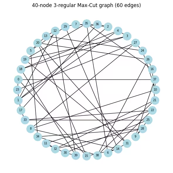
# A 3-regular graph (every node has exactly 3 neighbors) is a standard QAOA
N_LARGE = 40
G_large = nx.random_regular_graph(d=3, n=N_LARGE, seed=0)
edges_large = list(G_large.edges())
print(f"Graph: {N_LARGE} nodes, {len(edges_large)} edges (3-regular)")

# Visualize the graph so it is clear what problem we are solving before any
# quantum work. Nodes in a circular layout; each edge contributes +1 to the
# cut value when its endpoints land in different partitions.
pos_large = nx.circular_layout(G_large)
fig, ax = plt.subplots(figsize=(6, 6))
nx.draw(
    G_large,
    pos_large,
    with_labels=True,
    node_color="lightblue",
    node_size=400,
    font_size=7,
    ax=ax,
)
ax.set_title(f"40-node 3-regular Max-Cut graph ({len(edges_large)} edges)")
plt.tight_layout()
plt.show()

# Same Maxcut → OptimizationProblem → QUBO → Ising pipeline as the small example,
# applied to the 40-node graph.
prob_large = Maxcut(G_large).to_optimization_problem()
converter_large = OptimizationProblemToQubo()
qubo_large = converter_large.convert(prob_large)
cost_op_large, offset_large = to_ising(qubo_large)
n_qubits_large = cost_op_large.num_qubits
print(
    f"Cost operator: {n_qubits_large} qubits, {len(cost_op_large)} Pauli terms"
)

# ── Step 1b: QP relaxation (multi-start L-BFGS-B) ─────────────────────────
# Same multi-start approach as the small example. At 40 qubits the relaxed
# landscape has many more local minima, so 200 random starts are essential
# to find a low-energy warm-start point.
Q_large = qubo_large.objective.quadratic.to_array(symmetric=True)
mu_large = qubo_large.objective.linear.to_array()

def qp_obj_large(x):
    return x @ Q_large @ x + mu_large @ x + qubo_large.objective.constant

bounds_large = [(0.0, 1.0)] * n_qubits_large
rng_qp = np.random.default_rng(42)
best_val_large, c_star_large = np.inf, None

for _ in range(200):
    x0 = rng_qp.uniform(0.0, 1.0, n_qubits_large)
    res = minimize(qp_obj_large, x0, method="L-BFGS-B", bounds=bounds_large)
    if res.fun < best_val_large:
        best_val_large, c_star_large = res.fun, res.x

# Regularize and convert to rotation angles (same formula as small example)
epsilon_large = 0.25
c_clipped_large = np.clip(c_star_large, epsilon_large, 1 - epsilon_large)
thetas_large = 2 * np.arcsin(np.sqrt(c_clipped_large))
print(
    f"c* range: [{c_star_large.min():.3f}, {c_star_large.max():.3f}]  "
    f"theta range: [{thetas_large.min():.3f}, {thetas_large.max():.3f}] rad"
)

# Plot the distribution of c* values to see how much structure the relaxation
# extracted. Values near 0/1 mean confident assignments; values near 0.5 mean
# the classical solver was uncertain and quantum exploration is most needed there.
fig, ax = plt.subplots(figsize=(6, 3))
ax.hist(c_star_large, bins=20, color="steelblue", edgecolor="white")
ax.axvline(0.5, color="k", linestyle="--", label="Uniform prior (std QAOA)")
ax.set_xlabel(r"$c^*_i$")
ax.set_ylabel("Count")
ax.set_title(r"Distribution of warm-start values $c^*_i$ (40-node graph)")
ax.legend()
plt.tight_layout()
plt.show()

# ── Step 1c: Build WS-QAOA circuit ─────────────────────────────────────────
# Reuse build_ws_qaoa from the small-scale section unchanged; the helper
# scales automatically with n_qubits and the cost operator size.
p_large = 1
ws_qc_large, ws_gammas_large, ws_betas_large = build_ws_qaoa(
    cost_op_large, p_large, n_qubits_large, thetas_large
)
ws_qc_large.measure_all()

# ── Step 2: Transpile to hardware-native gates ──────────────────────────
# generate_preset_pass_manager compiles the abstract circuit to th
# gate set of the backend and inserts SWAP gates wherever the cost Hamiltonian
# couples qubits that are not directly connected on the processor.
pm = generate_preset_pass_manager(optimization_level=3, backend=backend)
ws_isa_large = pm.run(ws_qc_large)

ecr_count = ws_isa_large.count_ops().get("ecr", 0)
print(
    f"\nTranspiled circuit: 2Q depth={ws_isa_large.depth(lambda x: x.operation.num_qubits == 2)}"
)
ws_isa_large.draw("mpl", fold=-1)

Graph: 40 nodes, 60 edges (3-regular)

Output of the previous code cell

Cost operator: 40 qubits, 60 Pauli terms
c* range: [0.000, 1.000]  theta range: [1.047, 2.094] rad

Output of the previous code cell

Transpiled circuit: 2Q depth=86

Output of the previous code cell

# ── Classical baseline via simulated annealing ────────────────────
# Run SA before any hardware calls to get a strong classical reference cut
# value. SA is fast (seconds), needs no solver license, and reliably finds
# near-optimal solutions on 40-node graphs. We use sa_cut as the denominator
# for the approximation ratio instead of the looser QP upper bound.
#
# At each step we flip a random node and accept the move if it improves the
# cut, or with probability exp(delta/T) otherwise. Temperature T decays
# geometrically, allowing uphill moves early on to escape local minima.
def simulated_annealing_maxcut(
    G, seed=0, T0=2.0, T_min=1e-4, alpha=0.995, n_steps=100_000
):
    rng_sa = np.random.default_rng(seed)
    n = G.number_of_nodes()
    x = rng_sa.integers(0, 2, n)
    best_x = x.copy()
    best_cut = sum(1 for u, v in G.edges() if x[u] != x[v])
    T = T0
    for _ in range(n_steps):
        i = rng_sa.integers(0, n)
        delta = sum((-1 if x[i] != x[nb] else 1) for nb in G.neighbors(i))
        if delta > 0 or rng_sa.random() < np.exp(delta / T):
            x[i] ^= 1
            cut = sum(1 for u, v in G.edges() if x[u] != x[v])
            if cut > best_cut:
                best_cut, best_x = cut, x.copy()
        T = max(T * alpha, T_min)
    return best_x, best_cut

sa_solution, sa_cut = simulated_annealing_maxcut(G_large)
print(f"Simulated annealing cut value: {sa_cut}  (classical reference)")

# ── Step 3: Execution on hardware ───────────────────────────
# A Session reserves the backend so the COBYLA iterations and final sampling
# run back-to-back without re-queuing between jobs — important when the
# optimizer submits many short jobs sequentially. All jobs are tagged with
# "TUT_WSQAOA" for traceability in the IBM Quantum dashboard.
#
# EstimatorV2 with resilience_level=1 enables twirled readout error extinction
# (TREX), which corrects systematic measurement bit-flip errors without extra
# circuit overhead. 4096 shots per call balances estimation noise vs. job time.
estimator_options = EstimatorOptions()
estimator_options.resilience_level = 1
estimator_options.default_shots = 4096
estimator_options.environment.job_tags = ["TUT_WSQAOA"]

# Align the cost observable with the physical qubit layout chosen by the transpiler
cost_op_isa = cost_op_large.apply_layout(ws_isa_large.layout)
ws_param_order_isa = list(ws_isa_large.parameters)

ws_history_hw = []

with Session(backend=backend) as session:
    estimator_hw = Estimator(mode=session, options=estimator_options)

    def hw_cost_fn(params):
        bound = ws_isa_large.assign_parameters(
            dict(zip(ws_param_order_isa, params))
        )
        energy = (
            estimator_hw.run([(bound, cost_op_isa)]).result()[0].data.evs.real
        )
        ws_history_hw.append(float(energy))
        print(
            f"  iter {len(ws_history_hw):>3d}  <H_C> = {energy:.4f}", end="\r"
        )
        return float(energy)

    # Warm-start initialization: gamma=0 means the cost unitary is the identity on
    # the first call, so COBYLA immediately evaluates the warm-start state itself —
    # a much better starting signal than a random point.
    ws_params0_hw = np.concatenate(
        [np.zeros(p_large), np.full(p_large, np.pi / 4)]
    )

    ws_result_hw = minimize(
        hw_cost_fn,
        ws_params0_hw,
        method="COBYLA",
        options={"maxiter": 150, "rhobeg": 0.3},
    )
    print(
        f"\nOptimization complete: energy={ws_result_hw.fun:.4f}, "
        f"iterations={len(ws_history_hw)}"
    )

    # ── Step 3b: Sample the optimized circuit ──────────────────────────────────
    # Use 8192 shots for the final sample to get a reliable mode estimate.
    sampler_hw = Sampler(
        mode=session,
        options={"environment": {"job_tags": ["TUT_WSQAOA"]}},
    )
    ws_bound_hw = ws_isa_large.assign_parameters(
        dict(zip(ws_param_order_isa, ws_result_hw.x))
    )
    counts_hw = (
        sampler_hw.run([ws_bound_hw], shots=8192)
        .result()[0]
        .data.meas.get_counts()
    )

best_bs_hw = max(counts_hw, key=counts_hw.get)
best_count = counts_hw[best_bs_hw]
total_shots = sum(counts_hw.values())

# Decode: Qiskit returns bitstrings with qubit 0 at the rightmost position,
# so reversing the string maps character index i to variable x_i.
cut_val_hw, s0_hw, s1_hw = evaluate_cut(best_bs_hw[::-1], G_large)

# Compare against simulated annealing.
# A ratio >= 1.0 means WS-QAOA matched or beat the classical SA solution.
# A ratio close to 1.0 (e.g. > 0.95) shows the quantum result is competitive.
approx_ratio_hw = cut_val_hw / sa_cut
print(
    f"Most-probable bitstring frequency: {best_count}/{total_shots} "
    f"({100*best_count/total_shots:.1f}%)"
)
print(
    f"WS-QAOA cut: {cut_val_hw}  |  SA cut: {sa_cut}  "
    f"|  Approximation ratio vs SA: {approx_ratio_hw:.4f}"
)

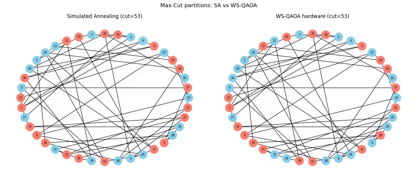
# Visualize both solutions side-by-side on the graph.
# Blue = partition S, orange = partition S-bar.
# Edges crossing between colors are the ones counted in the cut.
fig, axes = plt.subplots(1, 2, figsize=(14, 6))
for ax, assignment, cut, title in [
    (
        axes[0],
        list(sa_solution),
        sa_cut,
        f"Simulated Annealing (cut={sa_cut})",
    ),
    (
        axes[1],
        [int(b) for b in best_bs_hw[::-1]],
        cut_val_hw,
        f"WS-QAOA hardware (cut={cut_val_hw})",
    ),
]:
    colors = [
        "skyblue" if assignment[i] == 0 else "salmon" for i in G_large.nodes()
    ]
    nx.draw(
        G_large,
        pos_large,
        with_labels=True,
        node_color=colors,
        node_size=400,
        font_size=7,
        ax=ax,
    )
    ax.set_title(title)
plt.suptitle("Max-Cut partitions: SA vs WS-QAOA", fontsize=13)
plt.tight_layout()
plt.show()

# ── Step 4: Convergence plot and summary ──────────────────────────────────
# On real hardware the trace will be noisy (shot noise + gate errors), but the
# overall downward trend confirms that COBYLA is making progress despite noise.
fig, ax = plt.subplots(figsize=(7, 4))
ax.plot(ws_history_hw, color="tab:orange", label="WS-QAOA (hardware)")
ax.axhline(
    ws_result_hw.fun,
    color="tab:orange",
    linestyle=":",
    label=f"Final energy ({ws_result_hw.fun:.3f})",
)
ax.set_xlabel("Optimizer call")
ax.set_ylabel(r"$\langle H_C \rangle$")
ax.set_title(f"WS-QAOA convergence on {backend.name} (40 qubits, p=1)")
ax.legend()
plt.tight_layout()
plt.show()

print("\n=== Large Scale Summary ===")
print(f"{'Metric':<38} {'Value':>10}")
print("-" * 50)
print(f"{'Nodes / Edges':<38} {N_LARGE:>5} / {len(edges_large):<4}")
print(f"{'QAOA layers (p)':<38} {p_large:>10}")
print(f"{'Transpiled ECR gate count':<38} {ecr_count:>10}")
print(f"{'Transpiled circuit depth':<38} {ws_isa_large.depth():>10}")
print(f"{'Optimizer iterations':<38} {len(ws_history_hw):>10}")
print(f"{'WS-QAOA energy (hardware)':<38} {ws_result_hw.fun:>10.4f}")
print(f"{'Cut value':<38} {cut_val_hw:>10}")
print(f"{'Simulated annealing cut value':<38} {sa_cut:>10}")
print(f"{'Approximation ratio (vs SA)':<38} {approx_ratio_hw:>10.4f}")

Simulated annealing cut value: 53  (classical reference)
  iter  31  <H_C> = -12.4094
Optimization complete: energy=-13.0256, iterations=31
Most-probable bitstring frequency: 4/8192 (0.0%)
WS-QAOA cut: 53  |  SA cut: 53  |  Approximation ratio vs SA: 1.0000

Output of the previous code cell

=== Large Scale Summary ===
Metric                                      Value
--------------------------------------------------
Nodes / Edges                             40 / 60  
QAOA layers (p)                                 1
Transpiled ECR gate count                       0
Transpiled circuit depth                      276
Optimizer iterations                           31
WS-QAOA energy (hardware)                -13.0256
Cut value                                      53
Simulated annealing cut value                  53
Approximation ratio (vs SA)                1.0000

Langkah seterusnya

Cadangan

Jika anda mendapati kerja ini menarik, anda mungkin berminat dengan bahan berikut:

Lapisan QAOA yang lebih tinggi: Tingkatkan p untuk melihat bagaimana kedua-dua algoritma bertambah baik dengan lebih banyak lapisan litar, dan sama ada kelebihan WS-QAOA pada kedalaman rendah berterusan.
Qiskit addon optimization mapper: Terokai dokumentasi dan cuba memodelkan masalah gabungan yang berbeza, atau menggunakan penyelesai yang berbeza untuk pelonggaran berterusan.

Rujukan

[1] D. J. Egger, J. Mareček, and S. Woerner, "Warm-starting quantum optimization," Quantum, vol. 5, p. 479, 2021. arXiv:2009.10095

[2] E. Farhi, J. Goldstone, and S. Gutmann, "A quantum approximate optimization algorithm," arXiv:1411.4028, 2014.

Hasil pembelajaran​

Prasyarat​

Latar belakang​

Keperluan​

Persediaan​

Contoh simulator berskala kecil

Langkah 1: Petakan input klasik kepada masalah kuantum​

Langkah 2: Optimumkan masalah untuk pelaksanaan perkakasan kuantum​

Langkah 3: Laksanakan menggunakan primitif Qiskit​

Langkah 4: Pasca-proses dan kembalikan hasil dalam format klasik yang dikehendaki​

Contoh Perkakasan Berskala Besar

Langkah 1-4 dimampatkan menjadi satu blok kod​

Langkah seterusnya​

Rujukan​

Hasil pembelajaran

Prasyarat

Latar belakang

Keperluan

Persediaan

Langkah 1: Petakan input klasik kepada masalah kuantum

Langkah 2: Optimumkan masalah untuk pelaksanaan perkakasan kuantum

Langkah 3: Laksanakan menggunakan primitif Qiskit

Langkah 4: Pasca-proses dan kembalikan hasil dalam format klasik yang dikehendaki

Langkah 1-4 dimampatkan menjadi satu blok kod

Langkah seterusnya

Rujukan